12 Simple Linear Regression

Regression

Simple linear regression is a way of evaluating the relationship between two continuous variables. One variable is regarded as the predictor variable, explanatory variable, or independent variable ( ). The other variable is regarded as the response variable, outcome variable, or dependent variable.

For example, we might we interested in investigating the (linear?) relationship between:

heights and weights
high school grade point average and college grade point average
speed and gas mileage
outdoor temperature and evaporation rate
the Dow Jones industrial average and the consumer confidence index

Objectives

Upon completion of this lesson, you should be able to:

Formulate and interpret linear regression models for predicting outcomes based on one predictor variable,
Find the distribution of the least square parameters,
Conduct a hypothesis test or construct a confidence interval for the least square parameters, and
Construct a confidence interval or a conduct a hypothesis test for the correlation parameter $\rho$.

12.1 Types of Relationships

Before we dig into the methods of simple linear regression, we need to distinguish between two different type of relationships, namely:

deterministic relationships
statistical relationships

As we’ll soon see, simple linear regression concerns statistical relationships.

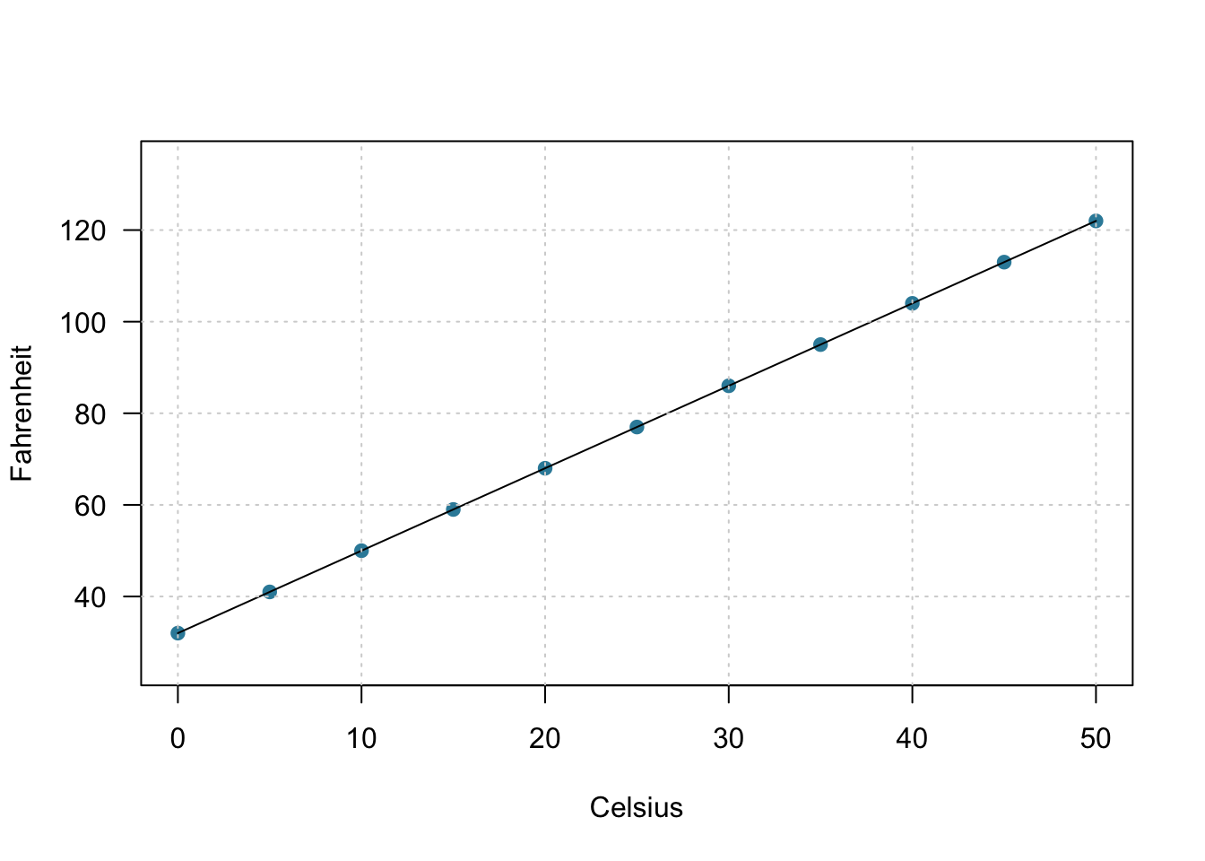
12.1.1 Deterministic (or Functional Relationships)

A deterministic (or functional) relationship is an exact relationship between the predictor $x$ and the response $y$. Take, for instance, the conversion relationship between temperature in degrees Celsius ($C$) and temperature in degrees Fahrenheit ($F$). We know the relationship is:

\[F=\dfrac{9}{5}C+32\]

Therefore, if we know that it is 10 degrees Celsius, we also know that it is 50 degrees Fahrenheit:

\[F=\dfrac{9}{5}(10)+32=50\]

This is what the exact (linear) relationship between degrees Celsius and degrees Fahrenheit looks like graphically:

Scatter plot of Fahrenheit vs Celsius with a connecting line — Fig 12.1

Other examples of deterministic relationships include…

the relationship between the diameter ($d$) and circumference of a circle ($C$): $C=\pi d$
the relationship between the applied weight ($X$) and the amount of stretch in a spring ($Y$) (known as Hooke’s Law): $Y=\alpha+\beta X$
the relationship between the voltage applied ($V$), the resistance ($r$) and the current ($I$) (known as Ohm’s Law): $I=\dfrac{V}{r}$
and, for a constant temperature, the relationship between pressure ($P$) and volume of gas ($V$) (known as Boyle’s Law): $P=\dfrac{\alpha}{V}$ where $\alpha$ is a known constant for each gas.

12.1.2 Statistical Relationships

A statistical relationship, on the other hand, is not an exact relationship. It is instead a relationship in which “trend” exists between the predictor $x$ and the response $y$, but there is also some “scatter.” Here’s a graph illustrating how a statistical relationship might look:

Scatter plot of skin cancer mortality versus state latitude with regression line — Fig 12.2

In this case, researchers investigated the relationship between the latitude (in degrees) at the center of each of the 50 U.S. states and the mortality (in deaths per 10 million) due to skin cancer in each of the 50 U.S. states. Perhaps we shouldn’t be surprised to see a downward trend, but not an exact relationship, between latitude and skin cancer mortality. That is, as the latitude increases for the northern states, in which sun exposure is less prevalent and less intense, mortality due to skin cancer decreases, but not perfectly so.

Other examples of statistical relationships include:

the positive relationship between height and weight
the positive relationship between alcohol consumed and blood alcohol content
the negative relationship between vital lung capacity and pack-years of smoking
the negative relationship between driving speed and gas mileage

It is these type of less-than-perfect statistical relationships that we are interested in when we investigate the methods of simple linear regression.

12.2 Least Squares: The Idea

Before delving into the theory of least squares, let’s motivate the idea behind the method of least squares by way of example.

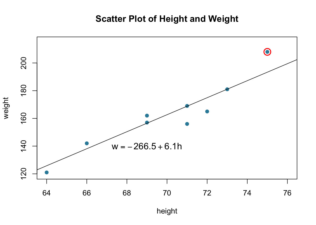
Example 12.1 A student was interested in quantifying the (linear) relationship between height (in inches) and weight (in pounds), so she measured the height and weight of ten randomly selected students in her class. After taking the measurements, she created the adjacent scatterplot of the obtained heights and weights. Wanting to summarize the relationship between height and weight, she eyeballed what she thought were two good lines (solid and dashed), but couldn’t decide between:

$\text{weight} = −266.5 + 6.1\times \text{height}$
$\text{weight} = −331.2 + 7.1\times \text{height}$

Which is the “best fitting line”?

Solution

In order to facilitate finding the best fitting line, let’s define some notation. Recalling that an experimental unit is the thing being measured (in this case, a student):

let $y_i$ denote the observed response for the $i^{th}$ experimental unit
let $x_i$ denote the predictor value for the $i^{th}$ experimental unit

-let $\hat{y}_i$ denote the predicted response (or fitted value) for the $i^{th}$ experimental unit

Therefore, for the data point circled in red:

Scatter Plot of Height and Weight from the student height and weight data set. — Fig 12.3: Scatter Plot of Height and Weight

we have:

\[x_i=75 \text{ and }y_i=208\]

And, using the unrounded version of the proposed line, the predicted weight of a randomly selected 75-inch tall student is:

\[\hat{y}_i=-266.534+6.13758(75)=193.8\text{ pounds}\]

Now, of course, the estimated line does not predict the weight of a 75-inch tall student perfectly. In this case, the prediction is 193.8 pounds, when the reality is 208 pounds. We have made an error in our prediction. That is, in using $\hat{y_i}$ to predict the actual response $y_i$ we make a prediction error (or a residual error) of size: \[ e_i=y_i-\hat{y}_i \] Now, a line that fits the data well will be one for which the $n$ prediction errors (one for each of the $n$ data points — $n=10$, in this case) are as small as possible in some overall sense. This idea is called the “least squares criterion.” In short, the least squares criterion tells us that in order to find the equation of the best fitting line:

\[\hat{y}_i=a_1+bx_i\]

we need to choose the values $a_1$ and $b$ that minimize the sum of the squared prediction errors. That is, find $a_1$ and $b$ that minimize:

\[Q=\sum\limits_{i=1}^n (y_i-\hat{y}_i)^2=\sum\limits_{i=1}^n (y_i-(a_1+bx_i))^2\]

So, using the least squares criterion to determine which of the two lines:

$\text{weight} = −266.5 + 6.1 \times\text{height}$
$\text{weight} = −331.2 + 7.1 \times \text{height}$

is the best fitting line, we just need to determine $Q$, the sum of the squared prediction errors for each of the two lines, and choose the line that has the smallest value of $Q$. For the dashed line, that is, for the line:

\[\text{weight} = −331.2 + 7.1\times\text{height}\]

here’s what the work would look like:

Table 12.1

$i$	$x_i$	$y_i$	$\hat{y}_i$	$(y_i - \hat{y}_i)$	$(y_i - \hat{y}_i)^2 $
1	63	127	116.1	10.9	118.8
2	64	121	123.2	-2.2	4.8
3	66	142	137.4	4.6	21.2
4	69	157	158.7	-1.7	2.9
5	69	162	158.7	3.3	10.9
6	71	156	172.9	-16.9	285.6
7	71	169	172.9	-3.9	15.2
8	72	165	180	-15	225.0
9	73	181	187.1	-6.1	37.2
10	75	208	201.3	6.7	44.9
Total					766.5

The first column labeled $i$ just keeps track of the index of the data points, $i=1, 2, \ldots, 10$. The columns labeled $x_i$ and $y_i$ contain the original data points. For example, the first student measured is 64 inches tall and weighs 121 pounds. The fourth column, labeled $\hat{y}_i$, contains the predicted weight of each student. For example, the predicted weight of the second student, who is 64 inches tall, is:

\[\hat{y}_1=-331.2+7.1(64)=123.2 \text{ pounds}\]

The fifth column contains the errors in using $\hat{y}_i$ to predict $y_i$. For the second student, the prediction error is:

\[e_1=121-123.3=-2.2\]

And, the last column contains the squared prediction errors. The squared prediction error for the second student is:

\[e^2_1=(-2.2)^2=4.84\]

By summing up the last column, that is, the column containing the squared prediction errors, we see that $Q=766.51$ for the dashed line. Now, for the solid line, that is, for the line:

\[\text{weight} = −266.5 + 6.1\times\text{height}\]

here’s what the work would look like:

Table 12.2

$i$	$x_i$	$y_i$	$\hat{y}_i$	$(y_i - \hat{y}_i)$	$(y_i - \hat{y}_i)^2 $
1	63	127	117.8	9.2	84.6
2	64	121	123.9	-2.9	8.4
3	66	142	136.1	5.9	34.8
4	69	157	154.4	2.6	6.8
5	69	162	154.4	7.6	57.8
6	71	156	166.6	-10.6	112.4
7	71	169	166.6	2.4	5.8
8	72	165	172.7	-7.7	59.3
9	73	181	178.8	2.2	4.8
10	75	208	191	17	289.0
Total					663.7

The calculations for each column are just as described previously. In this case, the sum of the last column, that is, the sum of the squared prediction errors for the solid line is $Q= 663.7$. Choosing the equation that minimizes $Q$, we can conclude that the solid line, that is:

\[\text{weight} = −266.5 + 6.1\times\text{height}\]

is the best fitting line.

In the preceding example, there’s one major problem with concluding that the solid line is the best fitting line! We’ve only considered two possible candidates. There are, in fact, an infinite number of possible candidates for best fitting line. The approach we used above clearly won’t work in practice. On the next page, we’ll instead derive some formulas for the slope and the intercept for least squares regression line.

12.3 Least Squares: The Theory

Now that we have the idea of least squares behind us, let’s make the method more practical by finding a formula for the intercept $a_1$ and slope $b$. We learned that in order to find the least squares regression line, we need to minimize the sum of the squared prediction errors, that is:

\[Q=\sum\limits_{i=1}^n (y_i-\hat{y}_i)^2\]

We just need to replace that $\hat{y}_i$ with the formula for the equation of a line:

\[\hat{y}_i=a_1+bx_i\]

to get:

\[Q=\sum\limits_{i=1}^n (y_i-\hat{y}_i)^2=\sum\limits_{i=1}^n (y_i-(a_1+bx_i))^2\]

We could go ahead and minimize $Q$ as such, but our textbook authors have opted to use a different form of the equation for a line, namely:

\[\hat{y}_i=a+b(x_i-\bar{x})\]

each form of the equation for a line has its advantages and disadvantages. Statistical software, such as R or Minitab, will typically calculate the least squares regression line using the form: \[\hat{y}_i=a_1+bx_i\]

Clearly a plus if you can get some computer to do the dirty work for you. A (minor) disadvantage of using this form of the equation, though, is that the intercept $a_1$ is the predicted value of the response $y$ when the predictor $x=0$, which is typically not very meaningful. For example, if $x$ is a student’s height (in inches) and $y$ is a student’s weight (in pounds), then the intercept is the predicted weight of a student who is 0 inches tall….. errrr…. you get the idea. On the other hand, if we use the equation:

\[\hat{y}_i=a+b(x_i-\bar{x})\]

then the intercept $a$ is the predicted value of the response $y$ when the predictor $x_i=\bar{x}$, that is, the average of the $x$ values. For example, if $x$ is a student’s height (in inches) and $y$ is a student’s weight (in pounds), then the intercept $a$ is the predicted weight of a student who is average in height. Much better, much more meaningful! The good news is that it is easy enough to get statistical software, such as R or Minitab, to calculate the least squares regression line in this form as well.

Okay, with that aside behind us, time to get to the punchline.

12.3.1 Least Squares Estimates

Note!
Lorem ipsum dolor sit amet, consectetur adipiscing elit, sed do eiusmod tempor incididunt ut labore et dolore magna aliqua. Ut enim ad minim veniam, quis nostrud exercitation ullamco laboris nisi ut aliquip ex ea commodo consequat. Duis aute irure dolor in reprehenderit in voluptate velit esse cillum dolore eu fugiat nulla pariatur. Excepteur sint occaecat cupidatat non proident, sunt in culpa qui officia deserunt mollit anim id est laborum. \[b=\dfrac{\sum\limits_{i=1}^n (x_i-\bar{x})y_i}{\sum\limits_{i=1}^n (x_i-\bar{x})^2}=\dfrac{\sum\limits_{i=1}^n x_iy_i-\left(\dfrac{1}{n}\right) \left(\sum\limits_{i=1}^n x_i\right) \left(\sum\limits_{i=1}^n y_i\right)}{\sum\limits_{i=1}^n x^2_i-\left(\dfrac{1}{n}\right) \left(\sum\limits_{i=1}^n x_i\right)^2}\]

Theorem 12.1 The least squares regression line is:

\[\hat{y}_i=a+b(x_i-\bar{x})\]

with least squares estimates:

\[a=\bar{y} \text{ and }b=\dfrac{\sum\limits_{i=1}^n (x_i-\bar{x})(y_i-\bar{y})}{\sum\limits_{i=1}^n (x_i-\bar{x})^2}\]

Proof

In order to derive the formulas for the intercept $a$ and slope $b$, we need to minimize:

\[Q=\sum\limits_{i=1}^n (y_i-(a+b(x_i-\bar{x})))^2\]

Time to put on your calculus cap, as minimizing $Q$ involves taking the derivative of $Q$ with respect to $a$ and $b$, setting to 0, and then solving for $a$ and $b$. Let’s do that. Starting with the derivative of $Q$ with respect to $a$, we get:

Video 12.1: Proof: Deriving the formulas for the intercept a and slope b

Now knowing that $a$ is $\bar{y}$, the average of the responses, let’s replace $a$ with $\bar{y}$ in the formula for $Q$:

\[Q=\sum\limits_{i=1}^n (y_i-(\bar{y}+b(x_i-\bar{x})))^2\]

and take the derivative of $Q$ with respect to $b$. Doing so, we get:

Video 12.2: Proof: Deriving formulas for the intercept and slope, Part 2

As was to be proved.

By the way, you might want to note that the only assumption relied on for the above calculations is that the relationship between the response $y$ and the predictor $x$ is linear.

Another thing you might note is that the formula for the slope $b$ is just fine providing you have statistical software to make the calculations. But, what would you do if you were stranded on a desert island, and were in need of finding the least squares regression line for the relationship between the depth of the tide and the time of day? You’d probably appreciate having a simpler calculation formula! You might also appreciate understanding the relationship between the slope $b$ and the sample correlation coefficient $r$.

With that lame motivation behind us, let’s derive alternative calculation formulas for the slope $b$.

Theorem 12.2 An alternative formula for the slope $b$ of the least squares regression line:

\[\hat{y}_i=a+b(x_i-\bar{x})\]

is:

\[b=\dfrac{\sum\limits_{i=1}^n (x_i-\bar{x})y_i}{\sum\limits_{i=1}^n (x_i-\bar{x})^2}=\dfrac{\sum\limits_{i=1}^n x_iy_i-\left(\dfrac{1}{n}\right) \left(\sum\limits_{i=1}^n x_i\right) \left(\sum\limits_{i=1}^n y_i\right)}{\sum\limits_{i=1}^n x^2_i-\left(\dfrac{1}{n}\right) \left(\sum\limits_{i=1}^n x_i\right)^2}\]

Proof

The proof, which may or may not show up on a quiz or exam, is left for you as an exercise.

12.4 The Model

12.4.1 What Do $a$ and $b$ Estimate?

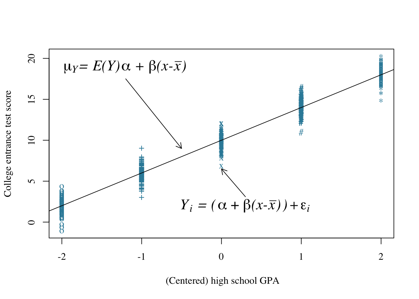
So far, we’ve formulated the idea, as well as the theory, behind least squares estimation. But, now we have a little problem. When we derived formulas for the least squares estimates of the intercept $a$ and the slope $b$, we never addressed for what parameters $a$ and $b$ serve as estimates. It is a crucial topic that deserves our attention. Let’s investigate the answer by considering the (linear) relationship between high school grade point averages (GPAs) and scores on a college entrance exam, such as the ACT exam. Well, let’s actually center the high school GPAs so that if $x$ denotes the high school GPA, then $x-\bar{x}$ is the centered high school GPA. Here’s what a plot of $x-\bar{x}$, the centered high school GPA, and $y$, the college entrance test score might look like:

Scatter plot of high school gpa vs college entrance test scores — Fig 12.4: High school gpa vs College entrance test scores

Well, okay, so that plot deserves some explanation:

Video 12.3: Example: Test scores and GPA, understanding the parameters

So far, in summary, we are assuming two things. First, among the entire population of college students, there is some unknown linear relationship between $\mu_y$, (or alternatively $E(Y)$), the average college entrance score, and $x-\bar{x}$, centered high school GPA. That is:

\[\mu_Y=E(Y)=\alpha+\beta(x-\bar{x})\]

Second, individual students deviate from the mean college entrance test score of the population of students having the same centered high school GPA by some unknown amount $\epsilon_i$. That is, if $Y_i$ denotes the college entrance test score for student $i$, then:

\[Y_i=\alpha+\beta(x-\bar{x})+\epsilon_i\]

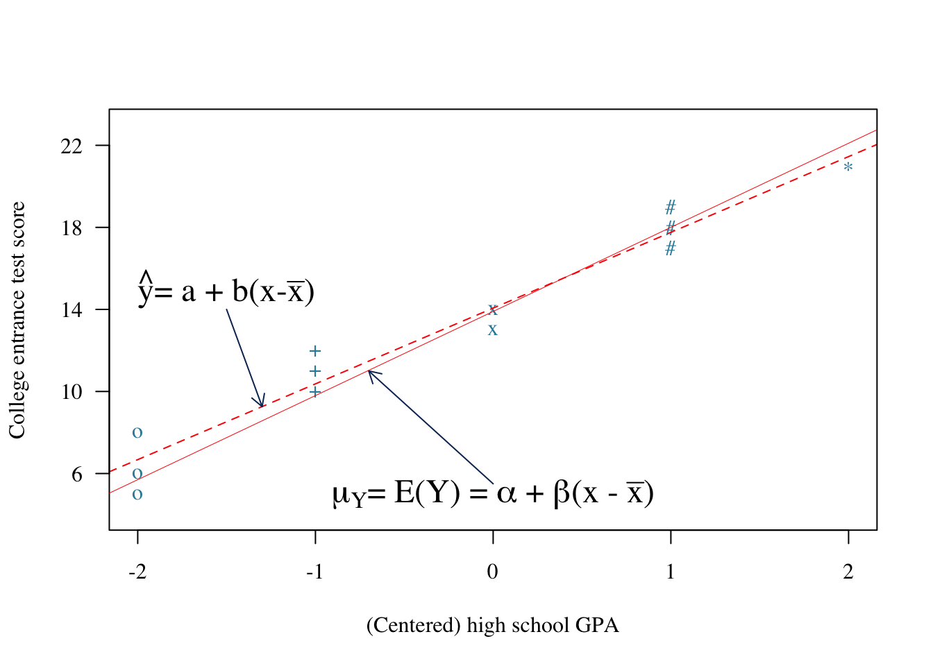
Unfortunately, we don’t have the luxury of collecting data on all of the college students in the population. So, we can never know the population intercept $\alpha$ or the population slope $\beta$. The best we can do is estimate $\alpha$ and $\beta$ by taking a random sample from the population of college students. Suppose we randomly select fifteen students from the population, in which three students have a centered high school GPA of −2, three students have a centered high school GPA of −1, and so on. We can use those fifteen data points to determine the best fitting (least squares) line:

\[\hat{y}_i=a+b(x_i-\bar{x})\]

Now, our least squares line isn’t going to be perfect, but it should do a pretty good job of estimating the true unknown population line:

Sample scatter plot of high school gpa vs college entrance test scores — Fig 12.5: Sample of High school gpa vs College entrance test scores

John: Fix the parameter equation above to match the old notes

That’s it in a nutshell. The intercept $a$ and the slope $b$ of the least squares regression line estimate, respectively, the intercept $\alpha$ and the slope $\beta$ of the unknown population line. The only assumption we make in doing so is that the relationship between the predictor $x$ and the response $y$ is linear.

Now, if we want to derive confidence intervals for $\alpha$ and $\beta$, as we are going to want to do on the next page, we are going to have to make a few more assumptions. That’s where the simple linear regression model comes to the rescue.

12.4.2 The Simple Linear Regression Model

So that we can have properly drawn normal curves, let’s borrow (steal?) an example from the textbook called Applied Linear Regression Models (4th edition, by Kutner, Nachtsheim, and Neter). Consider the relationship between $x$, the number of bids contracting companies prepare, and $y$, the number of hours it takes to prepare the bids:

Regression of line for hours vs number of bids — Fig 12.6

A couple of things to note about this graph. Note that again, the mean number of hours, $E(Y)$, is assumed to be linearly related to $X$, the number of bids prepared. That’s the first assumption. The textbook authors even go as far as to specify the values of typically unknown $\alpha$ and $\beta$. In this case, $\alpha$ is 9.5 and $\beta$ is 2.1.

Note that if $X=45$ bids are prepared, then the expected number of hours it took to prepare the bids is: \[ \mu_Y=E(Y)=9.5+2.1(45)=104 \] In one case, it took a contracting company 108 hours to prepare 45 bids. In that case, the error $\epsilon_i$ is 4. That is:

\[Y_i=108=E(Y)+\epsilon_i=104+4\]

The normal curves drawn for each value of $X$ are meant to suggest that the error terms $\epsilon_i$, and therefore the responses $Y_i$, are normally distributed. That’s a second assumption.

Did you also notice that the two normal curves in the plot are drawn to have the same shape? That suggests that each population (as defined by $X$) has a common variance. That’s a third assumption. That is, the errors, $\epsilon_i$, and therefore the responses $Y_i$, have equal variances for all $x$ values.

There’s one more assumption that is made that is difficult to depict on a graph. That’s the one that concerns the independence of the error terms. Let’s summarize!

In short, the simple linear regression model states that the following four conditions must hold:

The mean of the responses, $E(Y_i)$, is a $\textcolor{red}{L}$inear function of the $x_i$.
The errors, $\epsilon_i$, and hence the responses $Y_i$, are $\textcolor{red}{I}$ndependent.
The errors, $\epsilon_i$, and hence the responses $Y_i$, are $\textcolor{red}{N}$ormally distributed.
The errors, $\epsilon_i$, and hence the responses $Y_i$, have $\textcolor{red}{E}$qual variances ($\sigma^2$)) for all $x$ values.

Did you happen to notice that each of the four conditions is capitalized and emphasized in red? And, did you happen to notice that the capital letters spell $\textcolor{red}{L-I-N-E}$? Do you get it? We are investigating least squares regression lines, and the model effectively spells the word line! You might find this mnemonic an easy way to remember the four conditions.

12.4.3 Maximum Likelihood Estimates of $\alpha$ and $\beta$

We know that $a$ and $b$:

\[\displaystyle{a=\bar{y} \text{ and } b=\dfrac{\sum\limits_{i=1}^n (x_i-\bar{x})(y_i-\bar{y})}{\sum\limits_{i=1}^n (x_i-\bar{x})^2}}\]

are (“least squares”) estimators of $\alpha$ and $\beta$ that minimize the sum of the squared prediction errors. It turns out though that $a$ and $b$ are also maximum likelihood estimators of $\alpha$ and $\beta$ providing the four conditions of the simple linear regression model hold true.

Theorem 12.3 If the four conditions of the simple linear regression model hold true, then:

\[\displaystyle{a=\bar{y}\text{ and }b=\dfrac{\sum\limits_{i=1}^n (x_i-\bar{x})(y_i-\bar{y})}{\sum\limits_{i=1}^n (x_i-\bar{x})^2}}\]

are maximum likelihood estimators of $\alpha$ and $\beta$.

Proof

The simple linear regression model, in short, states that the errors $\epsilon_i$ are independent and normally distributed with mean 0 and variance $\sigma^2$. That is:

\[\epsilon_i \sim N(0,\sigma^2)\]

The linearity condition:

\[Y_i=\alpha+\beta(x_i-\bar{x})+\epsilon_i\]

therefore implies that:

\[Y_i \sim N(\alpha+\beta(x_i-\bar{x}),\sigma^2)\]

Therefore, the likelihood function is:

\[\displaystyle{L_{Y_i}(\alpha,\beta,\sigma^2)=\prod\limits_{i=1}^n \dfrac{1}{\sqrt{2\pi}\sigma} \text{exp}\left[-\dfrac{(Y_i-\alpha-\beta(x_i-\bar{x}))^2}{2\sigma^2}\right]}\]

which can be rewritten as:

\[\displaystyle{L=(2\pi)^{-n/2}(\sigma^2)^{-n/2}\text{exp}\left[-\dfrac{1}{2\sigma^2} \sum\limits_{i=1}^n (Y_i-\alpha-\beta(x_i-\bar{x}))^2\right]}\]

Taking the log of both sides, we get:

\[\displaystyle{\text{log}L=-\dfrac{n}{2}\text{log}(2\pi)-\dfrac{n}{2}\text{log}(\sigma^2)-\dfrac{1}{2\sigma^2} \sum\limits_{i=1}^n (Y_i-\alpha-\beta(x_i-\bar{x}))^2}\]

Now, that negative sign in front of that summation on the right hand side:

\[\color{black}\text{log}L=-\dfrac{n}{2} \text{log} (2\pi)-\dfrac{n}{2}\text{log}\left(\sigma^{2}\right)\color{blue}\boxed{\color{black}-}\color{black}\dfrac{1}{2\sigma^{2}} \color{blue}\boxed{\color{black}\sum\limits_{i=1}^{n}\left(Y_{i}-\alpha-\beta\left(x_{i}-\bar{x}\right)\right)^{2}}\]

tells us that the only way we can maximize $\log L(\alpha, \beta, \sigma^2)$ with respect to $\alpha$ and $\beta$ is if we minimize:

\[\displaystyle{a=\bar{y}\text{ and }b=\dfrac{\sum\limits_{i=1}^n (x_i-\bar{x})(y_i-\bar{y})}{\sum\limits_{i=1}^n (x_i-\bar{x})^2}}\]

are maximum likelihood estimators of $\alpha$ and $\beta$ under the assumption that the error terms are independent, normally distributed with mean 0 and variance $\sigma^2$. As was to be proved!

12.4.4 What About The (Unknown) Variance $\sigma^2$?

In short, the variance $\sigma^2$ quantifies how much the responses ($y$) vary around the (unknown) mean regression line $E(Y)$. Now, why should we care about the magnitude of the variance $\sigma^2$? The following example might help to illuminate the answer to that question.

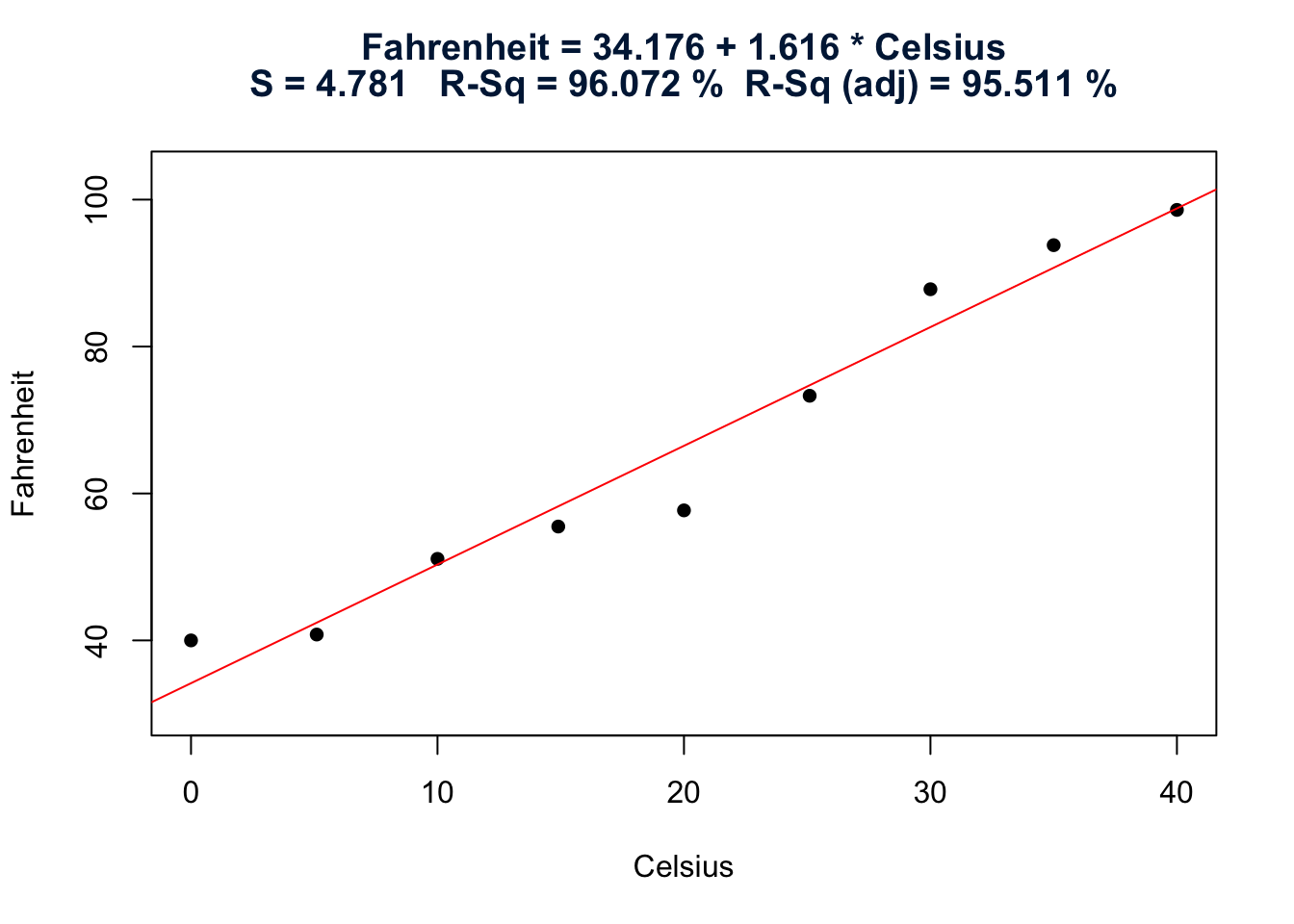
Example 12.2 We know that there is a perfect relationship between degrees Celsius ($C$) and degrees Fahrenheit ($F$), namely:

\[F=\dfrac{9}{5}C+32\]

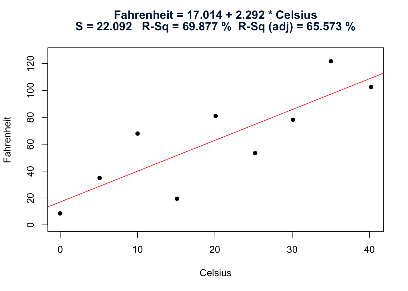
Suppose we are unfortunate, however, and therefore don’t know the relationship. We might attempt to learn about the relationship by collecting some temperature data and calculating a least squares regression line. When all is said and done, which brand of thermometers do you think would yield more precise future predictions of the temperature in Fahrenheit? The one whose data are plotted on the left? Or the one whose data are plotted on the right?

Scatter plot of Celsius vs Fahrenheit temperatures with regression line. — Fig 12.7

Scatter plot of Celsius vs Fahrenheit temperatures with regression line (with points more scattered) — Fig 12.8

Solution

As you can see, for the plot on the left, the Fahrenheit temperatures do not vary or “bounce” much around the estimated regression line. For the plot on the right, on the other hand, the Fahrenheit temperatures do vary or “bounce” quite a bit around the estimated regression line. It seems reasonable to conclude then that the brand of thermometers on the left will yield more precise future predictions of the temperature in Fahrenheit.

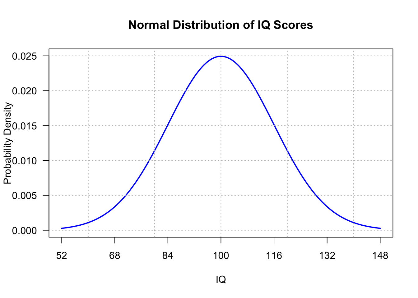
Now, the variance $\sigma^2$ is, of course, an unknown population parameter. The only way we can attempt to quantify the variance is to estimate it. In the case in which we had one population, say the (normal) population of IQ scores:

we would estimate the population variance $\sigma^2$ using the sample variance:

\[s^2=\dfrac{\sum\limits_{i=1}^n (Y_i-\bar{Y})^2}{n-1}\]

We have learned that $s^2$ is an unbiased estimator of $\sigma^2$, the variance of the one population. But what if we no longer have just one population, but instead have many populations? In our bids and hours example, there is a population for every value of $x$:

In this case, we have to estimate $\sigma^2$, the (common) variance of the many populations. There are two possibilities − one is a biased estimator, and one is an unbiased estimator.

Theorem 12.4 The maximum likelihood estimator of $\sigma^2$ is:

\[\hat{\sigma}^2=\dfrac{\sum\limits_{i=1}^n (Y_i-\hat{Y}_i)^2}{n}\]

It is a biased estimator of $\sigma^2$, the common variance of the many populations.

Proof

We have previously shown that the log of the likelihood function is:

\[\text{log}L=-\dfrac{n}{2}\text{log}(2\pi)-\dfrac{n}{2}\text{log}(\sigma^2)-\dfrac{1}{2\sigma^2} \sum\limits_{i=1}^n (Y_i-\alpha-\beta(x_i-\bar{x}))^2\]

To maximize the log likelihood, we have to take the partial derivative of the log likelihood with respect to $\sigma^2$. Doing so, we get:

\[\dfrac{\partial L_{Y_i}(\alpha,\beta,\sigma^2)}{\partial \sigma^2}=-\dfrac{n}{2\sigma^2}-\dfrac{1}{2}\sum (Y_i-\alpha-\beta(x_i-\bar{x}))^2 \cdot \left(- \dfrac{1}{(\sigma^2)^2}\right)\]

Setting the derivative equal to 0, and multiplying through by $2\sigma^4$:

\[\frac{\partial L_{Y_{i}}\left(\alpha, \beta, \sigma^{2}\right)}{\partial \sigma^{2}}=\left[-\frac{n}{2 \sigma^{2}}-\frac{1}{2} \sum\left(Y_{i}-\alpha-\beta\left(x_{i}-\bar{x}\right)\right)^{2} \cdot-\frac{1}{\left(\sigma^{2}\right)^{2}} \stackrel{\operatorname{SET}}{\equiv} 0\right] 2\left(\sigma^{2}\right)^{2}\]

we get:

\[-n\sigma^2+\sum (Y_i-\alpha-\beta(x_i-\bar{x}))^2 =0\]

And, solving for and putting a hat on $\sigma^2$, as well as replacing $\alpha$ and $\beta$ with their ML estimators, we get:

\[\hat{\sigma}^2=\dfrac{\sum (Y_i-\alpha-\beta(x_i-\bar{x}))^2 }{n}=\dfrac{\sum(Y_i-\hat{Y}_i)^2}{n}\]

As was to be proved.

Def. 12.1 (Mean Square Error) The mean square error, on the other hand:

\[MSE=\dfrac{\sum\limits_{i=1}^n(Y_i-\hat{Y}_i)^2}{n-2}\]

is an unbiased estimator of $\sigma^2$, the common variance of the many populations.

We’ll need to use these estimators of $\sigma^2$ when we derive confidence intervals for $\alpha$ and $\beta$ in the next section.

12.5 Confidence Intervals for Regression Parameters

Before we can derive confidence intervals for $\alpha$ and $\beta$, we first need to derive the probability distributions of $a$, $b$ and $\hat{\sigma}^2$. In the process of doing so, let’s adopt the more traditional estimator notation of putting a hat on greek letters. That is, here we’ll use:

\[a=\hat{\alpha} \text{ and }b=\hat{\beta}\]

Theorem 12.5 Under the assumptions of the simple linear regression model:

\[\hat{\alpha}\sim N\left(\alpha,\dfrac{\sigma^2}{n}\right)\]

Proof

Recall that the ML (and least squares!) estimator of $\alpha$ is:

\[a=\hat{\alpha}=\bar{Y}\]

where the responses $Y_i$ are independent and normally distributed. More specifically:

\[Y_i \sim N(\alpha+\beta(x_i-\bar{x}),\sigma^2)\]

The expected value of $\hat{\alpha}$ is $\alpha$, as shown here:

\[E(\hat{\alpha})=E(\bar{Y})=\frac{1}{n}\sum E(Y_i)=\frac{1}{n}\sum E(\alpha+\beta(x_i-\bar{x})=\frac{1}{n}\left[n\alpha+\beta \sum(x_i-\bar{x})\right]=\frac{1}{n}(n\alpha)=\alpha\]

Because $\sum (x_i-\bar{x})=0$.

The variance of $\hat{\alpha}$ follow directly from what we know about the variance of a sample mean, namely:

\[Var(\hat{\alpha})=Var(\bar{Y})=\dfrac{\sigma^2}{n}\]

Therefore, since a linear combination of normal random variables is also normally distributed, we have:

\[\hat{\alpha} \sim N\left(\alpha,\dfrac{\sigma^2}{n}\right)\]

as was to be proved!

Theorem 12.6 Under the assumptions of the simple linear regression model:

\[\hat{\beta}\sim N\left(\beta,\dfrac{\sigma^2}{\sum_{i=1}^n (x_i-\bar{x})^2}\right)\]

Proof

Recalling one of the shortcut formulas for the ML (and least squares!) estimator of $\beta$

\[b=\hat{\beta}=\dfrac{\sum_{i=1}^n (x_i-\bar{x})Y_i}{\sum_{i=1}^n (x_i-\bar{x})^2}\]

we see that the ML estimator is a linear combination of independent normal random variables $Y_i$ with:

\[Y_i \sim N(\alpha+\beta(x_i-\bar{x}),\sigma^2)\]

The expected value of $\hat{\beta}$ is $\beta$, as shown here:

\[E(\hat{\beta})=\frac{1}{\sum (x_i-\bar{x})^2}\sum E\left[(x_i-\bar{x})Y_i\right]=\frac{1}{\sum (x_i-\bar{x})^2}\sum (x_i-\bar{x})(\alpha +\beta(x_i-\bar{x}) =\frac{1}{\sum (x_i-\bar{x})^2}\left[ \alpha\sum (x_i-\bar{x}) +\beta \sum (x_i-\bar{x})^2 \right] \\=\beta\]

because $\sum (x_i-\bar{x})=0$.

And, the variance of $\hat{\beta}$ is:

\[\text{Var}(\hat{\beta})=\left[\frac{1}{\sum (x_i-\bar{x})^2}\right]^2\sum (x_i-\bar{x})^2(\text{Var}(Y_i))=\frac{\sigma^2}{\sum (x_i-\bar{x})^2}\]

Therefore, since a linear combination of normal random variables is also normally distributed, we have:

\[\hat{\beta}\sim N\left(\beta,\dfrac{\sigma^2}{\sum_{i=1}^n (x_i-\bar{x})^2}\right)\]

As was to be proved!

Theorem 12.7 Under the assumptions of the simple linear regression model:

\[\dfrac{n\hat{\sigma}^2}{\sigma^2}\sim \chi^2_{(n-2)}\]

and $a=\hat{\alpha}$, $b=\hat{\beta}$, and $\hat{\sigma}^2$ are mutually independent.

Argument

First, note that the heading here says Argument, not Proof. That’s because we are going to be doing some hand-waving and pointing to another reference, as the proof is beyond the scope of this course. That said, let’s start our hand-waving. For homework, you are asked to show that:

\[\sum\limits_{i=1}^n (Y_i-\alpha-\beta(x_i-\bar{x}))^2=n(\hat{\alpha}-\alpha)^2+(\hat{\beta}-\beta)^2\sum\limits_{i=1}^n (x_i-\bar{x})^2+\sum\limits_{i=1}^n (Y_i-\hat{Y})^2\]

Now, if we divide through both sides of the equation by the population variance $\sigma^2$, we get:

\[\dfrac{\sum_{i=1}^n (Y_i-\alpha-\beta(x_i-\bar{x}))^2 }{\sigma^2}=\dfrac{n(\hat{\alpha}-\alpha)^2}{\sigma^2}+\dfrac{(\hat{\beta}-\beta)^2\sum\limits_{i=1}^n (x_i-\bar{x})^2}{\sigma^2}+\dfrac{\sum (Y_i-\hat{Y})^2}{\sigma^2}\]

Rewriting a few of those terms just a bit, we get:

\[\dfrac{\sum_{i=1}^n (Y_i-\alpha-\beta(x_i-\bar{x}))^2 }{\sigma^2}=\dfrac{(\hat{\alpha}-\alpha)^2}{\sigma^2/n}+\dfrac{(\hat{\beta}-\beta)^2}{\sigma^2/\sum\limits_{i=1}^n (x_i-\bar{x})^2}+\dfrac{n\hat{\sigma}^2}{\sigma^2}\]

Now, the terms are written so that we should be able to readily identify the distributions of each of the terms. The distributions are:

\[\underbrace{\color{black}\frac{\sum\left(Y_{i}-\alpha-\beta\left(x_{i}-\bar{x}\right)\right)^{2}}{\sigma^2}}_{\underset{\text{}}{{\color{blue}x^2_{(n)}}}}=\underbrace{\color{black}\frac{(\hat{\alpha}-\alpha)^{2}}{\sigma^{2}/n}}_{\underset{\text{}}{{\color{blue}x^2_{(1)}}}}+\underbrace{\color{black}\frac{(\hat{\beta}-\beta)^{2}}{\sigma^{2}/\sum\left(x_{i}-\bar{x}\right)^{2}}}_{\underset{\text{}}{{\color{blue}x^2_{(1)}}}}+\underbrace{\color{black}\frac{n\hat{\sigma}^{2}}{\sigma^{2}}}_{\underset{\text{ }}{\color{red}\text{?}}}\]

Now, it might seem reasonable that the last term is a chi-square random variable with $n-2$ degrees of freedom. That is:

\[\dfrac{n\hat{\sigma}^2}{\sigma^2} \sim \chi^2_{(n-2)}\]

and furthermore, $a=\hat{\alpha}$, $b=\hat{\beta}$, and $\hat{\sigma^2}$ are mutually independent. (For a proof, you can refer to any number of mathematical statistics textbooks).

With the distributional results behind us, we can now derive $(1-\alpha)100\%$ confidence intervals for $\alpha$ and $\beta$!

Theorem 12.8 Under the assumptions of the simple linear regression model, a $(1-\alpha)100\%$ confidence interval for the slope parameter $\beta$ is:

\[b \pm t_{\alpha/2,n-2}\times \left(\dfrac{\sqrt{n}\hat{\sigma}}{\sqrt{n-2} \sqrt{\sum (x_i-\bar{x})^2}}\right)\]

or equivalently:

\[\hat{\beta} \pm t_{\alpha/2,n-2}\times \sqrt{\dfrac{MSE}{\sum (x_i-\bar{x})^2}}\] Proof

Recall the definition of a $T$ random variable. That is, recall that if:

$Z$ is a standard normal ($N(0,1)$)) random variable
$U$ is a chi-square random variable with $r$ degrees of freedom
$Z$ and $U$ are independent, then:

\[T=\dfrac{Z}{\sqrt{U/r}}\]

follows a $T$ distribution with $r$ degrees of freedom. Now, our work above tells us that:

\[\dfrac{\hat{\beta}-\beta}{\sigma/\sqrt{\sum (x_i-\bar{x})^2}} \sim N(0,1) \text{ and }\dfrac{n\hat{\sigma}^2}{\sigma^2} \sim \chi^2_{(n-2)} \text{ are independent}\]

Therefore, we have that:

\[T=\dfrac{\dfrac{\hat{\beta}-\beta}{\sigma/\sqrt{\sum (x_i-\bar{x})^2}}}{\sqrt{\dfrac{n\hat{\sigma}^2}{\sigma^2}/(n-2)}}=\dfrac{\hat{\beta}-\beta}{\sqrt{\dfrac{n\hat{\sigma}^2}{n-2}/\sum (x_i-\bar{x})^2}}=\dfrac{\hat{\beta}-\beta}{\sqrt{MSE/\sum (x_i-\bar{x})^2}} \sim t_{n-2}\]

follows a $T$ distribution with $n-2$ degrees of freedom. Now, deriving a confidence interval for $\beta$ reduces to the usual manipulation of the inside of a probability statement:

\[P\left(-t_{\alpha/2} \leq \dfrac{\hat{\beta}-\beta}{\sqrt{MSE/\sum (x_i-\bar{x})^2}} \leq t_{\alpha/2}\right)=1-\alpha\]

as was to be proved!

Now, for the confidence interval for the intercept parameter $\alpha$.

Theorem 12.9 Under the assumptions of the simple linear regression model, a $(1-\alpha)100\%$ confidence interval for the intercept parameter $\alpha$ is:

\[a \pm t_{\alpha/2,n-2}\times \left(\sqrt{\dfrac{\hat{\sigma}^2}{n-2}}\right)\]

or equivalently:

\[a \pm t_{\alpha/2,n-2}\times \left(\sqrt{\dfrac{MSE}{n}}\right)\]

Proof

The proof, which again may or may not appear on a future assessment, is left for you for practice.

Example 12.3 The following table shows $x$, the catches of Peruvian anchovies (in millions of metric tons) and $y$, the prices of fish meal (in current dollars per ton) for 14 consecutive years. (Data from Bardach, JE and Santerre, RM, Climate and the Fish in the Sea, Bioscience 31(3), 1981).

Row	Price	Catch
1	190	7.23
2	160	8.53
3	134	9.82
4	129	10.26
5	172	8.96
6	197	12.27
7	167	10.28
8	239	4.45
9	542	1.87
10	372	4.00
11	245	3.30
12	376	4.30
13	454	0.80
14	410	0.50

Find a 95% confidence interval for the slope parameter $\beta$.

Solution

The following portion of output was obtained using Minitab’s regression analysis package, with the parts useful to us here outlined ($\hat{\beta} = -29.39$ and $MSE = 5202$):

Regression Equation

Price = 452.3-29.39 Catch

Coefficients

Term	Coef	SE Coef	T-Value	P-Value	VIF
Constant	452.3	37.1	12.18	0.000
Catch	-29.39	5.13	-5.73	0.000	1.00

Model Summary

S	R-sq	R-sq(adj)	R-sq(pred)
72.1265	73.22%	70.98%	61.97%

Analysis of Variance

Source	DF	Adj SS	Adj MS	F-Value	P-Value
Regression	1	170655	170655	32.80	0.000
Catch	1	170655	170655	32.80	0.000
Error	12	62427	5202
Total	13	233082

Minitab’s basic descriptive analysis can also calculate the standard deviation of the $x$-values, 3.91, for us. Therefore, the formula for the sample variance tells us that:

\[\sum\limits_{i=1}^n (x_i-\bar{x})^2=(n-1)s^2=(13)(3.91)^2=198.7453\]

Putting the parts together, along with the fact that $t_{0.025, 12}=2.179$, we get:

\[-29.402 \pm 2.179 \sqrt{\dfrac{5139}{198.7453}}\]

which simplifies to: $-29.402 \pm 11.08.$ That is, we can be 95% confident that the slope parameter falls between −40.482 and −18.322. That is, we can be 95% confident that the average price of fish meal decreases between 18.322 and 40.482 dollars per ton for every one unit (one million metric ton) increase in the Peruvian anchovy catch.

Example 12.4 Find a 95% confidence interval for the intercept parameter $\alpha$.

Solution

We can use Minitab (or our calculator) to determine that the mean of the 14 responses is:

\[\dfrac{190+160+\cdots +410}{14}=270.5\]

Using that, as well as the $MSE = 5139$ obtained from the output above, along with the fact that $t_{0.025,12} = 2.179$, we get:

\[270.5 \pm 2.179 \sqrt{\dfrac{5139}{14}}\]

which simplifies to $270.5 \pm 41.75.$ That is, we can be 95% confident that the intercept parameter falls between 228.75 and 312.25 dollars per ton.

12.6 Hypothesis Tests Concerning Slope

Previously, we learned how to calculate point and interval estimates of the intercept and slope parameters, $\alpha$ and $\beta$, of a simple linear regression model:

\[Y_i=\alpha+\beta(x_i-\bar{x})+\epsilon_i\]

with the random errors $\epsilon_i$ following a normal distribution with mean 0 and variance $\sigma^2$. In this lesson, we’ll learn how to conduct a hypothesis test for testing the null hypothesis that the slope parameter equals some value, $\beta_0$, say. Specifically, we’ll learn how to test the null hypothesis $H_0:\beta=\beta_0$ using a $T$-statistic.

Once again we’ve already done the bulk of the theoretical work in developing a hypothesis test for the slope parameter $\beta$ of a simple linear regression model when we developed a $(1-\alpha)100\%$ confidence interval for $\beta$. We had shown then that:

\[T=\dfrac{\hat{\beta}-\beta}{\sqrt{\frac{MSE}{\sum(x_i-\bar{x})^2}}}\]

follows a $t_{n-2}$ distribution. Therefore, if we’re interested in testing the null hypothesis:

\[H_0:\beta=\beta_0\]

against any of the alternative hypotheses:

\[H_A:\beta > \beta_0, \qquad H_A:\beta < \beta_0,\qquad H_A:\beta \ne \beta_0\]

we can use the test statistic:

\[t=\dfrac{\hat{\beta}-\beta_0}{\sqrt{\frac{MSE}{\sum(x_i-\bar{x})^2}}}\]

and follow the standard hypothesis testing procedures.

12.7 Summary

This lesson covered the essentials of simple linear regression, a method to model linear relationships between a predictor (x) and response (y).

Key Takeaways include:

Model linear trends with scatter using the least squares method to find the best-fitting line.
Estimate intercept (a) and slope (b) to approximate population parameters $\alpha$ and $\beta$.
Assumptions (LINE): (L)inearity, (I)ndependence, (N)ormality, (E)qual variances.
Use confidence intervals and t-tests for inference on regression parameters.
Apply tools like R/Minitab to analyze real-world data and interpret results.

--- categories: [Regression] image: /assets/415lesson12thumb.png file-modified: --- # Simple Linear Regression Simple linear regression is a way of evaluating the relationship between two continuous variables. One variable is regarded as the predictor variable, explanatory variable, or independent variable ( ). The other variable is regarded as the response variable, outcome variable, or dependent variable. For example, we might we interested in investigating the (linear?) relationship between: - heights and weights - high school grade point average and college grade point average - speed and gas mileage - outdoor temperature and evaporation rate - the Dow Jones industrial average and the consumer confidence index ::: objectiveblock [Objectives]{.callout-header} Upon completion of this lesson, you should be able to: 1. Formulate and interpret linear regression models for predicting outcomes based on one predictor variable, 2. Find the distribution of the least square parameters, 3. Conduct a hypothesis test or construct a confidence interval for the least square parameters, and 4. Construct a confidence interval or a conduct a hypothesis test for the correlation parameter $\rho$. ::: ## Types of Relationships Before we dig into the methods of simple linear regression, we need to distinguish between two different type of relationships, namely: - deterministic relationships - statistical relationships As we'll soon see, simple linear regression concerns statistical relationships. ### Deterministic (or Functional Relationships) A **deterministic** (or **functional**) **relationship** is an exact relationship between the predictor $x$ and the response $y$. Take, for instance, the conversion relationship between temperature in degrees Celsius ($C$) and temperature in degrees Fahrenheit ($F$). We know the relationship is: $$F=\dfrac{9}{5}C+32$$ Therefore, if we know that it is 10 degrees Celsius, we also know that it is 50 degrees Fahrenheit: $$F=\dfrac{9}{5}(10)+32=50$$ This is what the exact (linear) relationship between degrees Celsius and degrees Fahrenheit looks like graphically: ```{r message=FALSE, warning=FALSE, error=FALSE, out.width="70%"} #| label: fig-lesson9_1 #| fig-alt: "Scatter plot of Fahrenheit vs Celsius with a connecting line" #| eval: true #| echo: false #| lightbox: true # Create data celsius <- seq(0, 50, by = 5) fahrenheit <- (celsius * 9/5) + 32 # Create scatter plot with line plot(celsius, fahrenheit, xlab = "Celsius", ylab = "Fahrenheit", xlim = c(0, 50), ylim = c(25, 135), pch = 19, # Solid circle points col = "#338BA8", # Blue points type = "p", las=1) # Points only lines(celsius, fahrenheit, col = "black") # Black line grid() # Add grid for clarity ``` Other examples of deterministic relationships include... * the relationship between the diameter ($d$) and circumference of a circle ($C$): $C=\pi d$ * the relationship between the applied weight ($X$) and the amount of stretch in a spring ($Y$) (known as Hooke's Law): $Y=\alpha+\beta X$ * the relationship between the voltage applied ($V$), the resistance ($r$) and the current ($I$) (known as Ohm's Law): $I=\dfrac{V}{r}$ * and, for a constant temperature, the relationship between pressure ($P$) and volume of gas ($V$) (known as Boyle's Law): $P=\dfrac{\alpha}{V}$ where $\alpha$ is a known constant for each gas. ### Statistical Relationships A **statistical relationship**, on the other hand, is not an exact relationship. It is instead a relationship in which "**trend**" exists between the predictor $x$ and the response $y$, but there is also some "**scatter**." Here's a graph illustrating how a statistical relationship might look: ```{r message=FALSE, warning=FALSE, error=FALSE, out.width="70%"} #| label: fig-skin-cancer #| fig-alt: "Scatter plot of skin cancer mortality versus state latitude with regression line" #| eval: true #| echo: false #| lightbox: true skincancer <- read.table("Data_files/skincancer.txt", header=T) #change to your file path attach(skincancer) model <- lm(Mort ~ Lat) plot(x=Lat, y=Mort, xlab="Latitude (at center of state)", ylab="Mortality (deaths per 10 million)", main="Skin Cancer Mortality versus State Latitude", col="#338BA8", pch=19, panel.last = lines(sort(Lat), fitted(model)[order(Lat)])) detach(skincancer) ``` In this case, researchers investigated the relationship between the latitude (in degrees) at the center of each of the 50 U.S. states and the mortality (in deaths per 10 million) due to skin cancer in each of the 50 U.S. states. Perhaps we shouldn't be surprised to see a downward trend, but not an exact relationship, between latitude and skin cancer mortality. That is, as the latitude increases for the northern states, in which sun exposure is less prevalent and less intense, mortality due to skin cancer decreases, but not perfectly so. Other examples of statistical relationships include: - the positive relationship between height and weight - the positive relationship between alcohol consumed and blood alcohol content - the negative relationship between vital lung capacity and pack-years of smoking - the negative relationship between driving speed and gas mileage It is these type of less-than-perfect statistical relationships that we are interested in when we investigate the methods of simple linear regression. ## Least Squares: The Idea Before delving into the theory of least squares, let's motivate the idea behind the method of least squares by way of example. ::: {#exm-leastsquares} A student was interested in quantifying the (linear) relationship between height (in inches) and weight (in pounds), so she measured the height and weight of ten randomly selected students in her class. After taking the measurements, she created the adjacent scatterplot of the obtained heights and weights. Wanting to summarize the relationship between height and weight, she eyeballed what she thought were two good lines (solid and dashed), but couldn't decide between: - $\text{weight} = −266.5 + 6.1\times \text{height}$ - $\text{weight} = −331.2 + 7.1\times \text{height}$ []{.bi .bi-question-circle-fill .fs-4 .text-success} **Which is the "best fitting line"?** ::: {.card .card-body .bg-light .ms-3 .mb-3 .pt-0} #### Solution In order to facilitate finding the best fitting line, let's define some notation. Recalling that an experimental unit is the thing being measured (in this case, a student): - let $y_i$ denote the **observed response** for the $i^{th}$ experimental unit - let $x_i$ denote the **predictor value** for the $i^{th}$ experimental unit -let $\hat{y}_i$ denote the **predicted response** (or **fitted value**) for the $i^{th}$ experimental unit Therefore, for the data point circled in red: ```{r eval="true" , fig.align="center", warning=FALSE, out.width="70%"} #| fig-alt: "Scatter Plot of Height and Weight from the student height and weight data set." #| fig-cap: "Scatter Plot of Height and Weight" #| fig-cap-location: bottom #| lightbox: True #| label: fig-htwt1 #| echo: false ht <- c(63, 64, 66, 69, 69, 71, 71, 72, 73, 75) wt <- c(127, 121, 142, 157, 162, 156, 169, 165, 181, 208) df <- data.frame(height = ht, weight = wt) plot(df$height, df$weight, xlab = "height", ylab = "weight", xlim = c(64, 76), ylim = c(120, 215), main = "Scatter Plot of Height and Weight", col="#338BA8", pch=19) # Adding a label to the line abline(a=-267, b = 6.138, col = "black") text(69, 140, expression(w == -266.5 + 6.1*h), col = "black", font = 2, cex = 1.2) # Identify and highlight the upper-right point (height = 75, weight = 208) points(75, 208, col = "red", pch = 1, cex = 2, lwd = 2) # Red circle around the point ``` we have: $$x_i=75 \text{ and }y_i=208$$ And, using the unrounded version of the proposed line, the predicted weight of a randomly selected 75-inch tall student is: $$\hat{y}_i=-266.534+6.13758(75)=193.8\text{ pounds}$$ Now, of course, the estimated line does not predict the weight of a 75-inch tall student perfectly. In this case, the prediction is 193.8 pounds, when the reality is 208 pounds. We have made an error in our prediction. That is, in using $\hat{y_i}$ to predict the actual response $y_i$ we make a **prediction error** (or a **residual error**) of size: $$ e_i=y_i-\hat{y}_i $$ Now, a line that fits the data well will be one for which the $n$ prediction errors (one for each of the $n$ data points — $n=10$, in this case) are as small as possible in some overall sense. This idea is called the "least squares criterion." In short, the **least squares criterion** tells us that in order to find the equation of the best fitting line: $$\hat{y}_i=a_1+bx_i$$ we need to choose the values $a_1$ and $b$ that minimize the sum of the squared prediction errors. That is, find $a_1$ and $b$ that minimize: $$Q=\sum\limits_{i=1}^n (y_i-\hat{y}_i)^2=\sum\limits_{i=1}^n (y_i-(a_1+bx_i))^2$$ So, using the least squares criterion to determine which of the two lines: - $\text{weight} = −266.5 + 6.1 \times\text{height}$ - $\text{weight} = −331.2 + 7.1 \times \text{height}$ is the best fitting line, we just need to determine $Q$, the sum of the squared prediction errors for each of the two lines, and choose the line that has the smallest value of $Q$. For the dashed line, that is, for the line: $$\text{weight} = −331.2 + 7.1\times\text{height}$$ here's what the work would look like: :::{.w-75 .mx-auto} ```{r, results='asis',echo=FALSE, message=FALSE} #| label: tbl-studenthtwt2 # Assuming dataset is your existing dataset in R # Install and load the kableExtra package if not already installed if (!requireNamespace("dplyr", quietly = TRUE)) { install.packages("dplyr") } if (!requireNamespace("kableExtra", quietly = TRUE)) { install.packages("kableExtra") } library(dplyr) library(kableExtra) student_ht_wt <- read.delim("data_files/student_height_weight.txt", col.names=c("x_i", "y_i")) student_ht_wt <- student_ht_wt %>% mutate(i = row_number()) student_ht_wt <- student_ht_wt %>% select(i, everything()) # Add a new column with the predicted values student_ht_wt$y_hat_i <- round(-331.2+7.1*student_ht_wt$x_i,1) student_ht_wt$y_diff <- round(student_ht_wt$y_i - student_ht_wt$y_hat_i,1) student_ht_wt$y_diff_squared <- round(student_ht_wt$y_diff^2,1) total_squared_diff <- sum(student_ht_wt$y_diff_squared) # Create a summary row with the total squared difference summary_row <- data.frame(i = "Total", x_i = "", y_i ="", y_hat_i = "", y_diff = "", y_diff_squared = total_squared_diff) student_ht_wt <- rbind(student_ht_wt, summary_row) # Display the updated table knitr::kable(student_ht_wt,col.names=c("\$i\$","\$x_i\$", "\$y_i\$","\$\\hat{y}_i\$","\$(y_i - \\hat{y}_i)\$","\$(y_i - \\hat{y}_i)^2 \$"), escape = FALSE, align="r") %>% kable_styling(full_width = FALSE,bootstrap_options = c("striped", "hover")) ``` ::: The first column labeled $i$ just keeps track of the index of the data points, $i=1, 2, \ldots, 10$. The columns labeled $x_i$ and $y_i$ contain the original data points. For example, the first student measured is 64 inches tall and weighs 121 pounds. The fourth column, labeled $\hat{y}_i$, contains the predicted weight of each student. For example, the predicted weight of the second student, who is 64 inches tall, is: $$\hat{y}_1=-331.2+7.1(64)=123.2 \text{ pounds}$$ The fifth column contains the errors in using $\hat{y}_i$ to predict $y_i$. For the second student, the prediction error is: $$e_1=121-123.3=-2.2$$ And, the last column contains the squared prediction errors. The squared prediction error for the second student is: $$e^2_1=(-2.2)^2=4.84$$ By summing up the last column, that is, the column containing the squared prediction errors, we see that $Q=766.51$ for the dashed line. Now, for the solid line, that is, for the line: $$\text{weight} = −266.5 + 6.1\times\text{height}$$ here's what the work would look like: :::{.w-75 .mx-auto} ```{r, results='asis',echo=FALSE, message=FALSE} #| label: tbl-studenthtwt3 # Assuming dataset is your existing dataset in R # Install and load the kableExtra package if not already installed if (!requireNamespace("dplyr", quietly = TRUE)) { install.packages("dplyr") } if (!requireNamespace("kableExtra", quietly = TRUE)) { install.packages("kableExtra") } library(dplyr) library(kableExtra) student_ht_wt <- read.delim("data_files/student_height_weight.txt", col.names=c("x_i", "y_i")) student_ht_wt <- student_ht_wt %>% mutate(i = row_number()) student_ht_wt <- student_ht_wt %>% select(i, everything()) # Add a new column with the predicted values student_ht_wt$y_hat_i <- round(-266.5+6.1*student_ht_wt$x_i,1) student_ht_wt$y_diff <- round(student_ht_wt$y_i - student_ht_wt$y_hat_i,1) student_ht_wt$y_diff_squared <- round(student_ht_wt$y_diff^2,1) total_squared_diff <- sum(student_ht_wt$y_diff_squared) # Create a summary row with the total squared difference summary_row <- data.frame(i = "Total", x_i = "", y_i ="", y_hat_i = "", y_diff = "", y_diff_squared = total_squared_diff) student_ht_wt <- rbind(student_ht_wt, summary_row) # Display the updated table knitr::kable(student_ht_wt,col.names=c("\$i\$","\$x_i\$", "\$y_i\$","\$\\hat{y}_i\$","\$(y_i - \\hat{y}_i)\$","\$(y_i - \\hat{y}_i)^2 \$"), escape = FALSE, align="r") %>% kable_styling(full_width = FALSE) ``` ::: The calculations for each column are just as described previously. In this case, the sum of the last column, that is, the sum of the squared prediction errors for the solid line is $Q= 663.7$. Choosing the equation that minimizes $Q$, we can conclude that the solid line, that is: $$\text{weight} = −266.5 + 6.1\times\text{height}$$ is the best fitting line. ::: ::: In the preceding example, there's one major problem with concluding that the solid line is the best fitting line! We've only considered two possible candidates. There are, in fact, an infinite number of possible candidates for best fitting line. The approach we used above clearly won't work in practice. On the next page, we'll instead derive some formulas for the slope and the intercept for least squares regression line. ## Least Squares: The Theory Now that we have the idea of least squares behind us, let's make the method more practical by finding a formula for the intercept $a_1$ and slope $b$. We learned that in order to find the least squares regression line, we need to minimize the sum of the squared prediction errors, that is: $$Q=\sum\limits_{i=1}^n (y_i-\hat{y}_i)^2$$ We just need to replace that $\hat{y}_i$ with the formula for the equation of a line: $$\hat{y}_i=a_1+bx_i$$ to get: $$Q=\sum\limits_{i=1}^n (y_i-\hat{y}_i)^2=\sum\limits_{i=1}^n (y_i-(a_1+bx_i))^2$$ We could go ahead and minimize $Q$ as such, but our textbook authors have opted to use a different form of the equation for a line, namely: $$\hat{y}_i=a+b(x_i-\bar{x})$$ each form of the equation for a line has its advantages and disadvantages. Statistical software, such as R or Minitab, will typically calculate the least squares regression line using the form: $$\hat{y}_i=a_1+bx_i$$ Clearly a plus if you can get some computer to do the dirty work for you. A (minor) disadvantage of using this form of the equation, though, is that the intercept $a_1$ is the predicted value of the response $y$ when the predictor $x=0$, which is typically not very meaningful. For example, if $x$ is a student's height (in inches) and $y$ is a student's weight (in pounds), then the intercept is the predicted weight of a student who is 0 inches tall..... errrr.... you get the idea. On the other hand, if we use the equation: $$\hat{y}_i=a+b(x_i-\bar{x})$$ then the intercept $a$ is the predicted value of the response $y$ when the predictor $x_i=\bar{x}$, that is, the average of the $x$ values. For example, if $x$ is a student's height (in inches) and $y$ is a student's weight (in pounds), then the intercept $a$ is the predicted weight of a student who is average in height. Much better, much more meaningful! The good news is that it is easy enough to get statistical software, such as R or Minitab, to calculate the least squares regression line in this form as well. Okay, with that aside behind us, time to get to the punchline. ### Least Squares Estimates ::: {.callout-caution appearance="minimal"} **Note!** \ Lorem ipsum dolor sit amet, consectetur adipiscing elit, sed do eiusmod tempor incididunt ut labore et dolore magna aliqua. Ut enim ad minim veniam, quis nostrud exercitation ullamco laboris nisi ut aliquip ex ea commodo consequat. Duis aute irure dolor in reprehenderit in voluptate velit esse cillum dolore eu fugiat nulla pariatur. Excepteur sint occaecat cupidatat non proident, sunt in culpa qui officia deserunt mollit anim id est laborum. $$b=\dfrac{\sum\limits_{i=1}^n (x_i-\bar{x})y_i}{\sum\limits_{i=1}^n (x_i-\bar{x})^2}=\dfrac{\sum\limits_{i=1}^n x_iy_i-\left(\dfrac{1}{n}\right) \left(\sum\limits_{i=1}^n x_i\right) \left(\sum\limits_{i=1}^n y_i\right)}{\sum\limits_{i=1}^n x^2_i-\left(\dfrac{1}{n}\right) \left(\sum\limits_{i=1}^n x_i\right)^2}$$ ::: :::: {.callout-note appearance="minimal"} ::: {#thm-lsrline} The **least squares regression line** is: $$\hat{y}_i=a+b(x_i-\bar{x})$$ with **least squares estimates**: $$a=\bar{y} \text{ and }b=\dfrac{\sum\limits_{i=1}^n (x_i-\bar{x})(y_i-\bar{y})}{\sum\limits_{i=1}^n (x_i-\bar{x})^2}$$ **Proof** In order to derive the formulas for the intercept $a$ and slope $b$, we need to minimize: $$Q=\sum\limits_{i=1}^n (y_i-(a+b(x_i-\bar{x})))^2$$ Time to put on your calculus cap, as minimizing $Q$ involves taking the derivative of $Q$ with respect to $a$ and $b$, setting to 0, and then solving for $a$ and $b$. Let's do that. Starting with the derivative of $Q$ with respect to $a$, we get: :::{.w-75 .mx-auto #vid-lsr1 } {{< video https://youtu.be/oAaPR1qVedw >}} Proof: Deriving the formulas for the intercept a and slope b ::: Now knowing that $a$ is $\bar{y}$, the average of the responses, let's replace $a$ with $\bar{y}$ in the formula for $Q$: $$Q=\sum\limits_{i=1}^n (y_i-(\bar{y}+b(x_i-\bar{x})))^2$$ and take the derivative of $Q$ with respect to $b$. Doing so, we get: :::{.w-75 .mx-auto #vid-lsr2 } {{< video https://youtu.be/pWMp1vhStDE >}} Proof: Deriving formulas for the intercept and slope, Part 2 ::: As was to be proved. ::: :::: By the way, you might want to note that the only assumption relied on for the above calculations is that the relationship between the response $y$ and the predictor $x$ is linear. Another thing you might note is that the formula for the slope $b$ is just fine providing you have statistical software to make the calculations. But, what would you do if you were stranded on a desert island, and were in need of finding the least squares regression line for the relationship between the depth of the tide and the time of day? You'd probably appreciate having a simpler calculation formula! You might also appreciate understanding the relationship between the slope $b$ and the sample correlation coefficient $r$. With that lame motivation behind us, let's derive alternative calculation formulas for the slope $b$. :::: {.callout-note appearance="minimal"} ::: {#thm-lsralt} An alternative formula for the slope $b$ of the least squares regression line: $$\hat{y}_i=a+b(x_i-\bar{x})$$ is: $$b=\dfrac{\sum\limits_{i=1}^n (x_i-\bar{x})y_i}{\sum\limits_{i=1}^n (x_i-\bar{x})^2}=\dfrac{\sum\limits_{i=1}^n x_iy_i-\left(\dfrac{1}{n}\right) \left(\sum\limits_{i=1}^n x_i\right) \left(\sum\limits_{i=1}^n y_i\right)}{\sum\limits_{i=1}^n x^2_i-\left(\dfrac{1}{n}\right) \left(\sum\limits_{i=1}^n x_i\right)^2}$$ **Proof** The proof, which may or may not show up on a quiz or exam, is left for you as an exercise. ::: :::: ## The Model ### What Do $a$ and $b$ Estimate? So far, we've formulated the idea, as well as the theory, behind least squares estimation. But, now we have a little problem. When we derived formulas for the least squares estimates of the intercept $a$ and the slope $b$, we never addressed for what parameters $a$ and $b$ serve as estimates. It is a crucial topic that deserves our attention. Let's investigate the answer by considering the (linear) relationship between high school grade point averages (GPAs) and scores on a college entrance exam, such as the ACT exam. Well, let's actually center the high school GPAs so that if $x$ denotes the high school GPA, then $x-\bar{x}$ is the centered high school GPA. Here's what a plot of $x-\bar{x}$, the centered high school GPA, and $y$, the college entrance test score might look like: ```{r fig.align="center",out.width="70%"} #| label: fig-gpavsentrance3 #| fig-alt: Scatter plot of high school gpa vs college entrance test scores #| fig-cap: High school gpa vs College entrance test scores #| eval: true #| echo: false #| lightbox: true # Set font to serif (similar to Times New Roman) par(family = "serif") rm(list=ls()) set.seed(789) # Create X with five clusters: 0, 1, 2, 3, 4 X <- c(rep(0, 100), rep(1, 100), rep(2, 100), rep(3, 100), rep(4, 100)) # Transform X to map 0,1,2,3,4 to -2,-1,0,1,2 X_centered <- X - 2 Y <- 2 + 4*X + rnorm(500, 0, 1) # Define pch values for each cluster (-2, -1, 0, 1, 2) pch_values <- rep(c("o", "+", "x", "#","*"), each = 100) # Open circle, filled circle, triangle, square, diamond plot(X_centered, Y, xlab = " (Centered) high school GPA", ylab = "College entrance test score", main = "", col = "#338BA8", # Set points to blue pch = as.character(pch_values)) # Different symbols for each cluster # Adjust intercept: a = 2 + 4 * 2 = 10 abline(a = 10, b = 4, col = "black") exp1 <- expression(paste(italic(Y[i]), italic(" = ("),italic(alpha), " + ", italic(beta), italic("(x-"),italic(bar(x)),italic(")"),italic(")"),italic("+"), italic(epsilon[i]), sep="")) text(0.3, 2, exp1, col = "black", font=3, cex=1.5) arrows(x0 = 0.3, y0 = 3.1, x1 = 0, y1 = 6.5, col = "black", lwd = 1, length = 0.1) exp2 <- expression(italic(paste(mu[Y], "= E(Y)", alpha, " + ", beta, "(x-",bar(x),")", sep=""))) text(-1.2, 19, exp2, col = "black", font=3, cex=1.5) arrows(x0 = -1.2, y0 = 17.5, x1 = -0.5, y1 = 9, col = "black", lwd = 1, length = 0.1) ``` Well, okay, so that plot deserves some explanation: :::{.w-75 .mx-auto #vid- } {{< video https://youtu.be/mdzP-v6vl74 >}} Example: Test scores and GPA, understanding the parameters ::: So far, in summary, we are assuming two things. First, among the entire population of college students, there is some unknown linear relationship between $\mu_y$, (or alternatively $E(Y)$), the average college entrance score, and $x-\bar{x}$, centered high school GPA. That is: $$\mu_Y=E(Y)=\alpha+\beta(x-\bar{x})$$ Second, individual students deviate from the mean college entrance test score of the population of students having the same centered high school GPA by some unknown amount $\epsilon_i$. That is, if $Y_i$ denotes the college entrance test score for student $i$, then: $$Y_i=\alpha+\beta(x-\bar{x})+\epsilon_i$$ Unfortunately, we don't have the luxury of collecting data on all of the college students in the population. So, we can never know the population intercept $\alpha$ or the population slope $\beta$. The best we can do is estimate $\alpha$ and $\beta$ by taking a random sample from the population of college students. Suppose we randomly select fifteen students from the population, in which three students have a centered high school GPA of −2, three students have a centered high school GPA of −1, and so on. We can use those fifteen data points to determine the best fitting (least squares) line: $$\hat{y}_i=a+b(x_i-\bar{x})$$ Now, our least squares line isn't going to be perfect, but it should do a pretty good job of estimating the true unknown population line: ```{r message=FALSE, warning=FALSE, error=FALSE, out.width="70%"} #| label: fig-samplegpaentrance4 #| fig-alt: Sample scatter plot of high school gpa vs college entrance test scores #| fig-cap: Sample of High school gpa vs College entrance test scores #| eval: true #| echo: false #| lightbox: true par(family = "serif") rm(list=ls()) # Clear workspace # cat("\014") # Clear console (optional) # Define your dataset data <- data.frame( X = c(-2, -2, -2, -1, -1, -1, 0, 0, 1, 1, 1, 2), Y = c(8, 6, 5, 12, 11, 10, 13, 14, 19, 18, 17, 21) ) # Define shapes for each unique X value pch_values <- c("o", "+", "x", "#","*") # Shapes for X = -2, -1, 0, 1, 2 pch <- sapply(data$X, function(val) pch_values[which(c(-2, -1, 0, 1, 2) == val)]) # Fit a linear model model <- lm(Y ~ X, data = data) # Plot the data plot(data$X, data$Y, ylim = c(4, 23), yaxt = "n", xlab="(Centered) high school GPA", ylab="College entrance test score", pch = pch, col = "#338BA8", cex = 1, panel.last = { abline(model, col = "red", lty = 2) # Add regression line }) # Add theoretical line equation exp1 <- expression(paste(mu[Y], "= E(Y) = ", alpha, " + ", beta, "(x - ", bar(x), ")", sep="")) text(0, 5, exp1, col = "black", font=2, cex=1.5) arrows(x0 = 0, y0 = 5.5, x1 = -.7, y1 = 11, col = "#093162", lwd = 1, length = 0.1) # Add fitted line equation exp2 <- expression(paste(hat(y), "= ", a, " + ", b, "(x","-",bar(x),")", sep="")) text(-1.5, 15, exp2, col = "black", font=2, cex=1.5) arrows(x0 = -1.5, y0 = 14, x1 = -1.3, y1 = predict(model, data.frame(X=-1.3)), col = "#093162", lwd = 1, length = 0.1) abline(a = 13.9, b = 4.1, col = "red", lty = 1, lwd = .5) axis(2, at = seq(6, 22, by = 4), las=1) ``` ::: {.callout-important} ## John: Fix the parameter equation above to match the old notes ::: That's it in a nutshell. The intercept $a$ and the slope $b$ of the least squares regression line estimate, respectively, the intercept $\alpha$ and the slope $\beta$ of the unknown population line. The only assumption we make in doing so is that the relationship between the predictor $x$ and the response $y$ is linear. Now, if we want to derive confidence intervals for $\alpha$ and $\beta$, as we are going to want to do on the next page, we are going to have to make a few more assumptions. That's where the simple linear regression model comes to the rescue. ### The Simple Linear Regression Model So that we can have properly drawn normal curves, let's borrow (steal?) an example from the textbook called Applied Linear Regression Models (4th edition, by Kutner, Nachtsheim, and Neter). Consider the relationship between $x$, the number of bids contracting companies prepare, and $y$, the number of hours it takes to prepare the bids: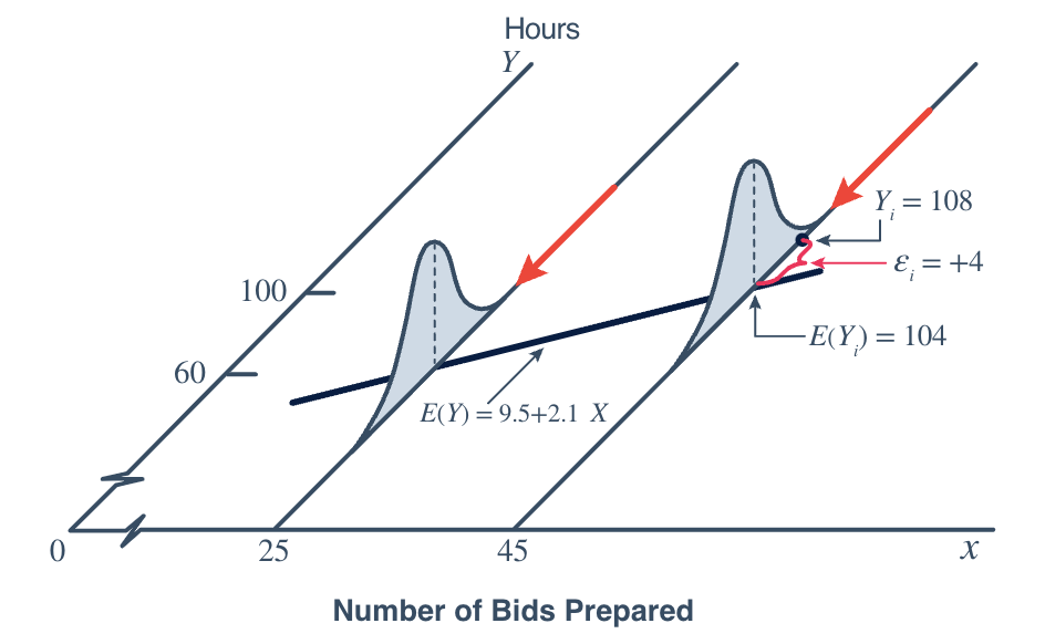 ![ ](assets/lesson9_11.png){#fig-bidsgraph fig-alt="Regression of line for hours vs number of bids" fig-scap="A statistical graph showing the relationship between the number of bids prepared (X-axis, 0 to 45) and hours (Y-axis, 0 to 100). The graph includes two dashed probability density curves peaking around 25 and 45 bids, with a line labeled E(Y) = 9.5 + 2.1X. At 45 bids, annotations indicate Y_i = 108, ε_i = +4, and E(Y_i) = 104." .mx-auto .d-block width="60%" .lightbox} A couple of things to note about this graph. Note that again, the mean number of hours, $E(Y)$, is assumed to be **linearly related** to $X$, the number of bids prepared. That's the first assumption. The textbook authors even go as far as to specify the values of typically unknown $\alpha$ and $\beta$. In this case, $\alpha$ is 9.5 and $\beta$ is 2.1. Note that if $X=45$ bids are prepared, then the expected number of hours it took to prepare the bids is: $$ \mu_Y=E(Y)=9.5+2.1(45)=104 $$ In one case, it took a contracting company 108 hours to prepare 45 bids. In that case, the error $\epsilon_i$ is 4. That is: $$Y_i=108=E(Y)+\epsilon_i=104+4$$ The normal curves drawn for each value of $X$ are meant to suggest that the error terms $\epsilon_i$, and therefore the responses $Y_i$, are **normally distributed**. That's a second assumption. Did you also notice that the two normal curves in the plot are drawn to have the same shape? That suggests that each population (as defined by $X$) has a common variance. That's a third assumption. That is, the errors, $\epsilon_i$, and therefore the responses $Y_i$, have **equal variances** for all $x$ values. There's one more assumption that is made that is difficult to depict on a graph. That's the one that concerns the **independence** of the error terms. Let's summarize! In short, the simple linear regression model states that the following four conditions must hold: - The mean of the responses, $E(Y_i)$, is a $\textcolor{red}{L}$inear function of the $x_i$. - The errors, $\epsilon_i$, and hence the responses $Y_i$, are $\textcolor{red}{I}$ndependent. - The errors, $\epsilon_i$, and hence the responses $Y_i$, are $\textcolor{red}{N}$ormally distributed. - The errors, $\epsilon_i$, and hence the responses $Y_i$, have $\textcolor{red}{E}$qual variances ($\sigma^2$)) for all $x$ values. Did you happen to notice that each of the four conditions is capitalized and emphasized in red? And, did you happen to notice that the capital letters spell $\textcolor{red}{L-I-N-E}$? Do you get it? We are investigating least squares regression lines, and the model effectively spells the word line! You might find this mnemonic an easy way to remember the four conditions. ### Maximum Likelihood Estimates of $\alpha$ and $\beta$ We know that $a$ and $b$: $$\displaystyle{a=\bar{y} \text{ and } b=\dfrac{\sum\limits_{i=1}^n (x_i-\bar{x})(y_i-\bar{y})}{\sum\limits_{i=1}^n (x_i-\bar{x})^2}}$$ are ("least squares") estimators of $\alpha$ and $\beta$ that minimize the sum of the squared prediction errors. It turns out though that $a$ and $b$ are also maximum likelihood estimators of $\alpha$ and $\beta$ **providing the four conditions of the simple linear regression model hold true.** :::{.callout-note appearance="minimal"} :::{#thm-lsrMLE} If the four conditions of the simple linear regression model hold true, then: $$\displaystyle{a=\bar{y}\text{ and }b=\dfrac{\sum\limits_{i=1}^n (x_i-\bar{x})(y_i-\bar{y})}{\sum\limits_{i=1}^n (x_i-\bar{x})^2}}$$ are maximum likelihood estimators of $\alpha$ and $\beta$. **Proof** The simple linear regression model, in short, states that the errors $\epsilon_i$ are independent and normally distributed with mean 0 and variance $\sigma^2$. That is: $$\epsilon_i \sim N(0,\sigma^2)$$ The linearity condition: $$Y_i=\alpha+\beta(x_i-\bar{x})+\epsilon_i$$ therefore implies that: $$Y_i \sim N(\alpha+\beta(x_i-\bar{x}),\sigma^2)$$ Therefore, the likelihood function is: $$\displaystyle{L_{Y_i}(\alpha,\beta,\sigma^2)=\prod\limits_{i=1}^n \dfrac{1}{\sqrt{2\pi}\sigma} \text{exp}\left[-\dfrac{(Y_i-\alpha-\beta(x_i-\bar{x}))^2}{2\sigma^2}\right]}$$ which can be rewritten as: $$\displaystyle{L=(2\pi)^{-n/2}(\sigma^2)^{-n/2}\text{exp}\left[-\dfrac{1}{2\sigma^2} \sum\limits_{i=1}^n (Y_i-\alpha-\beta(x_i-\bar{x}))^2\right]}$$ Taking the log of both sides, we get: $$\displaystyle{\text{log}L=-\dfrac{n}{2}\text{log}(2\pi)-\dfrac{n}{2}\text{log}(\sigma^2)-\dfrac{1}{2\sigma^2} \sum\limits_{i=1}^n (Y_i-\alpha-\beta(x_i-\bar{x}))^2}$$ Now, that negative sign in front of that summation on the right hand side: $$\color{black}\text{log}L=-\dfrac{n}{2} \text{log} (2\pi)-\dfrac{n}{2}\text{log}\left(\sigma^{2}\right)\color{blue}\boxed{\color{black}-}\color{black}\dfrac{1}{2\sigma^{2}} \color{blue}\boxed{\color{black}\sum\limits_{i=1}^{n}\left(Y_{i}-\alpha-\beta\left(x_{i}-\bar{x}\right)\right)^{2}}$$ tells us that the only way we can maximize $\log L(\alpha, \beta, \sigma^2)$ with respect to $\alpha$ and $\beta$ is if we minimize: $$\displaystyle{a=\bar{y}\text{ and }b=\dfrac{\sum\limits_{i=1}^n (x_i-\bar{x})(y_i-\bar{y})}{\sum\limits_{i=1}^n (x_i-\bar{x})^2}}$$ are maximum likelihood estimators of $\alpha$ and $\beta$ under the assumption that the error terms are independent, normally distributed with mean 0 and variance $\sigma^2$. As was to be proved! ::: :::: ### What About The (Unknown) Variance $\sigma^2$? In short, the variance $\sigma^2$ quantifies how much the responses ($y$) vary around the (unknown) mean regression line $E(Y)$. Now, why should we care about the magnitude of the variance $\sigma^2$? The following example might help to illuminate the answer to that question. ::: {#exm-degrees} We know that there is a perfect relationship between degrees Celsius ($C$) and degrees Fahrenheit ($F$), namely: $$F=\dfrac{9}{5}C+32$$ Suppose we are unfortunate, however, and therefore don't know the relationship. We might attempt to learn about the relationship by collecting some temperature data and calculating a least squares regression line. When all is said and done, which brand of thermometers do you think would yield more precise future predictions of the temperature in Fahrenheit? The one whose data are plotted on the left? Or the one whose data are plotted on the right? ::: {.grid} ::: {.g-col-lg-6 .g-col-md-6 .g-col-sm-12} ```{r message=FALSE, warning=FALSE, error=FALSE, out.width="90%"} #| label: fig-scattertemp #| fig-alt: Scatter plot of Celsius vs Fahrenheit temperatures with regression line. #| eval: true #| echo: false #| lightbox: true # Create a data frame with the given data data <- data.frame( celsius = c(0.0, 5.1, 10.0, 14.9, 20.0, 25.1, 30.0, 35.0, 40.0), fahrenheit = c(40.0, 40.8, 51.1, 55.5, 57.7, 73.3, 87.8, 93.8, 98.6) ) # Create a linear regression model with fahrenheit as the response and celsius as the explanatory variable model_celsius_to_fahrenheit <- lm(fahrenheit ~ celsius, data = data) # Create the scatterplot plot(data$celsius, data$fahrenheit, xlab = "Celsius", ylab = "Fahrenheit", pch = 16, col = "black", # pch = 16 for solid dots ylim = c(30, max(data$fahrenheit) + 5)) # Start y-axis at 30, extend to max(fahrenheit) + 5 for padding # Add the regression line abline(model_celsius_to_fahrenheit, col = "red") # Extract regression equation, S, R-Sq, and R-Sq (adj) equation <- paste("Fahrenheit =", round(coef(model_celsius_to_fahrenheit)[1], 3), "+", round(coef(model_celsius_to_fahrenheit)[2], 3), "* Celsius") s_value <- round(summary(model_celsius_to_fahrenheit)$sigma, 3) rsq <- round(summary(model_celsius_to_fahrenheit)$r.squared * 100, 3) # Convert to percentage rsq_adj <- round(summary(model_celsius_to_fahrenheit)$adj.r.squared * 100, 3) # Convert to percentage # Add title with equation, S, R-Sq, and R-Sq (adj) title(main = c(equation, paste("S =", s_value, " R-Sq =", rsq, "% R-Sq (adj) =", rsq_adj, "%")), line = 2, col.main = "#001e44") ``` ::: ::: {.g-col-lg-6 .g-col-md-6 .g-col-sm-12} ```{r message=FALSE, warning=FALSE, error=FALSE, out.width="90%"} #| label: fig-scattertemp2 #| fig-alt: Scatter plot of Celsius vs Fahrenheit temperatures with regression line (with points more scattered) #| eval: true #| echo: false #| lightbox: true # Create a data frame with the given data data <- data.frame( celsius = c(0.0,5.1,10.0,20.1,15.1,25.2,30.1,35.0,40.2), fahrenheit = c(8.5,34.9,67.9,81.1,19.4,53.4,78.2,121.7,102.5) ) # Create a linear regression model with fahrenheit as the response and celsius as the explanatory variable model_celsius_to_fahrenheit <- lm(fahrenheit ~ celsius, data = data) # Create the scatterplot plot(data$celsius, data$fahrenheit, xlab = "Celsius", ylab = "Fahrenheit", pch = 16, col = "black", # pch = 16 for solid dots ylim = c(0, max(data$fahrenheit) + 5)) # Start y-axis at 0, extend to max(fahrenheit) + 5 for padding # Add the regression line abline(model_celsius_to_fahrenheit, col = "red") # Extract regression equation, S, R-Sq, and R-Sq (adj) equation <- paste("Fahrenheit =", round(coef(model_celsius_to_fahrenheit)[1], 3), "+", round(coef(model_celsius_to_fahrenheit)[2], 3), "* Celsius") s_value <- round(summary(model_celsius_to_fahrenheit)$sigma, 3) rsq <- round(summary(model_celsius_to_fahrenheit)$r.squared * 100, 3) # Convert to percentage rsq_adj <- round(summary(model_celsius_to_fahrenheit)$adj.r.squared * 100, 3) # Convert to percentage # Add title with equation, S, R-Sq, and R-Sq (adj) title(main = c(equation, paste("S =", s_value, " R-Sq =", rsq, "% R-Sq (adj) =", rsq_adj, "%")), line = 2, col.main = "#001e44") ``` ::: ::: ::: {.card .card-body .bg-light .ms-3 .mb-3 .pt-0} #### Solution As you can see, for the plot on the left, the Fahrenheit temperatures do not vary or "bounce" much around the estimated regression line. For the plot on the right, on the other hand, the Fahrenheit temperatures do vary or "bounce" quite a bit around the estimated regression line. It seems reasonable to conclude then that the brand of thermometers on the left will yield more precise future predictions of the temperature in Fahrenheit. Now, the variance $\sigma^2$ is, of course, an unknown population parameter. The only way we can attempt to quantify the variance is to estimate it. In the case in which we had one population, say the (normal) population of IQ scores: ```{r message=FALSE, warning=FALSE, error=FALSE, out.width="70%"} #| label: fig-iqnormal #| fig-alt: Normal curve of IQ scores #| eval: true #| echo: false #| lightbox: true # Define parameters for the normal distribution mean_iq <- 100 # Mean of IQ distribution sd_iq <- 16 # Standard deviation (adjust if needed) # Create a sequence of IQ values for smooth plotting x <- seq(52, 148, length.out = 1000) # Fine grid for smooth curve # Calculate the probability density for each x value y <- dnorm(x, mean = mean_iq, sd = sd_iq) # Create the plot plot(x, y, type = "l", # Line plot for the curve xlab = "IQ", # X-axis label ylab = "Probability Density", # Y-axis label xaxt = "n", # Suppress default x-axis yaxt = "n", # Suppress default y-axis xlim = c(52, 148), # X-axis range ylim = c(0, 0.025), # Y-axis range main = "Normal Distribution of IQ Scores", # Plot title col = "blue", # Curve color lwd = 2, las=1) # Line width # Add custom x-axis with ticks at 52, 68, 84, 100, 116, 132, 148 axis(1, at = seq(52, 148, by = 16)) # Add custom y-axis with ticks at 0.000, 0.005, 0.010, ..., 0.025 axis(2, at = seq(0, 0.025, by = 0.005), las=1) # Add grid lines (optional, for clarity) grid(nx = NULL, ny = NULL, col = "gray", lty = "dotted") ``` we would estimate the population variance $\sigma^2$ using the sample variance: $$s^2=\dfrac{\sum\limits_{i=1}^n (Y_i-\bar{Y})^2}{n-1}$$ We have learned that $s^2$ is an unbiased estimator of $\sigma^2$, the variance of the one population. But what if we no longer have just one population, but instead have many populations? In our bids and hours example, there is a population for every value of $x$: ![ ](assets/lesson9_11.png){#fig-bidsgraph fig-alt="Regression of line for hours vs number of bids" fig-scap="A statistical graph showing the relationship between the number of bids prepared (X-axis, 0 to 45) and hours (Y-axis, 0 to 100). The graph includes two dashed probability density curves peaking around 25 and 45 bids, with a line labeled E(Y) = 9.5 + 2.1X. At 45 bids, annotations indicate Y_i = 108, ε_i = +4, and E(Y_i) = 104." .mx-auto .d-block width="60%" .lightbox} In this case, we have to estimate $\sigma^2$, the (common) variance of the many populations. There are two possibilities − one is a biased estimator, and one is an unbiased estimator. ::: ::: :::{.callout-note appearance="minimal"} :::{#thm-lsrMLE2} The maximum likelihood estimator of $\sigma^2$ is: $$\hat{\sigma}^2=\dfrac{\sum\limits_{i=1}^n (Y_i-\hat{Y}_i)^2}{n}$$ It is a biased estimator of $\sigma^2$, the common variance of the **many** populations. **Proof** We have previously shown that the log of the likelihood function is: $$\text{log}L=-\dfrac{n}{2}\text{log}(2\pi)-\dfrac{n}{2}\text{log}(\sigma^2)-\dfrac{1}{2\sigma^2} \sum\limits_{i=1}^n (Y_i-\alpha-\beta(x_i-\bar{x}))^2$$ To maximize the log likelihood, we have to take the partial derivative of the log likelihood with respect to $\sigma^2$. Doing so, we get: $$\dfrac{\partial L_{Y_i}(\alpha,\beta,\sigma^2)}{\partial \sigma^2}=-\dfrac{n}{2\sigma^2}-\dfrac{1}{2}\sum (Y_i-\alpha-\beta(x_i-\bar{x}))^2 \cdot \left(- \dfrac{1}{(\sigma^2)^2}\right)$$ Setting the derivative equal to 0, and multiplying through by $2\sigma^4$: $$\frac{\partial L_{Y_{i}}\left(\alpha, \beta, \sigma^{2}\right)}{\partial \sigma^{2}}=\left[-\frac{n}{2 \sigma^{2}}-\frac{1}{2} \sum\left(Y_{i}-\alpha-\beta\left(x_{i}-\bar{x}\right)\right)^{2} \cdot-\frac{1}{\left(\sigma^{2}\right)^{2}} \stackrel{\operatorname{SET}}{\equiv} 0\right] 2\left(\sigma^{2}\right)^{2}$$ we get: $$-n\sigma^2+\sum (Y_i-\alpha-\beta(x_i-\bar{x}))^2 =0$$ And, solving for and putting a hat on $\sigma^2$, as well as replacing $\alpha$ and $\beta$ with their ML estimators, we get: $$\hat{\sigma}^2=\dfrac{\sum (Y_i-\alpha-\beta(x_i-\bar{x}))^2 }{n}=\dfrac{\sum(Y_i-\hat{Y}_i)^2}{n}$$ As was to be proved. ::: :::: ::: {#def-name .ms-3} ### Mean Square Error The **mean square error**, on the other hand: $$MSE=\dfrac{\sum\limits_{i=1}^n(Y_i-\hat{Y}_i)^2}{n-2}$$ is an **unbiased estimator** of $\sigma^2$, the common variance of the **many** populations. ::: We'll need to use these estimators of $\sigma^2$ when we derive confidence intervals for $\alpha$ and $\beta$ in the next section. ## Confidence Intervals for Regression Parameters Before we can derive confidence intervals for $\alpha$ and $\beta$, we first need to derive the probability distributions of $a$, $b$ and $\hat{\sigma}^2$. In the process of doing so, let's adopt the more traditional estimator notation of putting a hat on greek letters. That is, here we'll use: $$a=\hat{\alpha} \text{ and }b=\hat{\beta}$$ ::: {.callout-note appearance="minimal"} ::: {#thm-lsrprobdist} Under the assumptions of the simple linear regression model: $$\hat{\alpha}\sim N\left(\alpha,\dfrac{\sigma^2}{n}\right)$$ **Proof** Recall that the ML (and least squares!) estimator of $\alpha$ is: $$a=\hat{\alpha}=\bar{Y}$$ where the responses $Y_i$ are independent and normally distributed. More specifically: $$Y_i \sim N(\alpha+\beta(x_i-\bar{x}),\sigma^2)$$ The expected value of $\hat{\alpha}$ is $\alpha$, as shown here: $$E(\hat{\alpha})=E(\bar{Y})=\frac{1}{n}\sum E(Y_i)=\frac{1}{n}\sum E(\alpha+\beta(x_i-\bar{x})=\frac{1}{n}\left[n\alpha+\beta \sum(x_i-\bar{x})\right]=\frac{1}{n}(n\alpha)=\alpha$$ Because $\sum (x_i-\bar{x})=0$. The variance of $\hat{\alpha}$ follow directly from what we know about the variance of a sample mean, namely: $$Var(\hat{\alpha})=Var(\bar{Y})=\dfrac{\sigma^2}{n}$$ Therefore, since a linear combination of normal random variables is also normally distributed, we have: $$\hat{\alpha} \sim N\left(\alpha,\dfrac{\sigma^2}{n}\right)$$ as was to be proved! ::: ::: ::: {.callout-note appearance="minimal"} ::: {#thm-lsrvariance} Under the assumptions of the simple linear regression model: $$\hat{\beta}\sim N\left(\beta,\dfrac{\sigma^2}{\sum_{i=1}^n (x_i-\bar{x})^2}\right)$$ **Proof** Recalling one of the shortcut formulas for the ML (and least squares!) estimator of $\beta$ $$b=\hat{\beta}=\dfrac{\sum_{i=1}^n (x_i-\bar{x})Y_i}{\sum_{i=1}^n (x_i-\bar{x})^2}$$ we see that the ML estimator is a linear combination of independent normal random variables $Y_i$ with: $$Y_i \sim N(\alpha+\beta(x_i-\bar{x}),\sigma^2)$$ The expected value of $\hat{\beta}$ is $\beta$, as shown here: $$E(\hat{\beta})=\frac{1}{\sum (x_i-\bar{x})^2}\sum E\left[(x_i-\bar{x})Y_i\right]=\frac{1}{\sum (x_i-\bar{x})^2}\sum (x_i-\bar{x})(\alpha +\beta(x_i-\bar{x}) =\frac{1}{\sum (x_i-\bar{x})^2}\left[ \alpha\sum (x_i-\bar{x}) +\beta \sum (x_i-\bar{x})^2 \right] \\=\beta$$ because $\sum (x_i-\bar{x})=0$. And, the variance of $\hat{\beta}$ is: $$\text{Var}(\hat{\beta})=\left[\frac{1}{\sum (x_i-\bar{x})^2}\right]^2\sum (x_i-\bar{x})^2(\text{Var}(Y_i))=\frac{\sigma^2}{\sum (x_i-\bar{x})^2}$$ Therefore, since a linear combination of normal random variables is also normally distributed, we have: $$\hat{\beta}\sim N\left(\beta,\dfrac{\sigma^2}{\sum_{i=1}^n (x_i-\bar{x})^2}\right)$$ As was to be proved! ::: :::: ::: {.callout-note appearance="minimal"} ::: {#thm-lsrindependent} Under the assumptions of the simple linear regression model: $$\dfrac{n\hat{\sigma}^2}{\sigma^2}\sim \chi^2_{(n-2)}$$ and $a=\hat{\alpha}$, $b=\hat{\beta}$, and $\hat{\sigma}^2$ are mutually independent. **Argument** First, note that the heading here says Argument, not Proof. That's because we are going to be doing some hand-waving and pointing to another reference, as the proof is beyond the scope of this course. That said, let's start our hand-waving. For homework, you are asked to show that: $$\sum\limits_{i=1}^n (Y_i-\alpha-\beta(x_i-\bar{x}))^2=n(\hat{\alpha}-\alpha)^2+(\hat{\beta}-\beta)^2\sum\limits_{i=1}^n (x_i-\bar{x})^2+\sum\limits_{i=1}^n (Y_i-\hat{Y})^2$$ Now, if we divide through both sides of the equation by the population variance $\sigma^2$, we get: $$\dfrac{\sum_{i=1}^n (Y_i-\alpha-\beta(x_i-\bar{x}))^2 }{\sigma^2}=\dfrac{n(\hat{\alpha}-\alpha)^2}{\sigma^2}+\dfrac{(\hat{\beta}-\beta)^2\sum\limits_{i=1}^n (x_i-\bar{x})^2}{\sigma^2}+\dfrac{\sum (Y_i-\hat{Y})^2}{\sigma^2}$$ Rewriting a few of those terms just a bit, we get: $$\dfrac{\sum_{i=1}^n (Y_i-\alpha-\beta(x_i-\bar{x}))^2 }{\sigma^2}=\dfrac{(\hat{\alpha}-\alpha)^2}{\sigma^2/n}+\dfrac{(\hat{\beta}-\beta)^2}{\sigma^2/\sum\limits_{i=1}^n (x_i-\bar{x})^2}+\dfrac{n\hat{\sigma}^2}{\sigma^2}$$ Now, the terms are written so that we should be able to readily identify the distributions of each of the terms. The distributions are: $$\underbrace{\color{black}\frac{\sum\left(Y_{i}-\alpha-\beta\left(x_{i}-\bar{x}\right)\right)^{2}}{\sigma^2}}_{\underset{\text{}}{{\color{blue}x^2_{(n)}}}}=\underbrace{\color{black}\frac{(\hat{\alpha}-\alpha)^{2}}{\sigma^{2}/n}}_{\underset{\text{}}{{\color{blue}x^2_{(1)}}}}+\underbrace{\color{black}\frac{(\hat{\beta}-\beta)^{2}}{\sigma^{2}/\sum\left(x_{i}-\bar{x}\right)^{2}}}_{\underset{\text{}}{{\color{blue}x^2_{(1)}}}}+\underbrace{\color{black}\frac{n\hat{\sigma}^{2}}{\sigma^{2}}}_{\underset{\text{ }}{\color{red}\text{?}}}$$ Now, it might seem reasonable that the last term is a chi-square random variable with $n-2$ degrees of freedom. That is: $$\dfrac{n\hat{\sigma}^2}{\sigma^2} \sim \chi^2_{(n-2)}$$ and furthermore, $a=\hat{\alpha}$, $b=\hat{\beta}$, and $\hat{\sigma^2}$ are mutually independent. (For a proof, you can refer to any number of mathematical statistics textbooks). With the distributional results behind us, we can now derive $(1-\alpha)100\%$ confidence intervals for $\alpha$ and $\beta$! ::: :::: ::: {.callout-note appearance="minimal"} ::: {#thm-cislope} Under the assumptions of the simple linear regression model, a $(1-\alpha)100\%$ **confidence interval for the slope parameter** $\beta$ is: $$b \pm t_{\alpha/2,n-2}\times \left(\dfrac{\sqrt{n}\hat{\sigma}}{\sqrt{n-2} \sqrt{\sum (x_i-\bar{x})^2}}\right)$$ or equivalently: $$\hat{\beta} \pm t_{\alpha/2,n-2}\times \sqrt{\dfrac{MSE}{\sum (x_i-\bar{x})^2}}$$ **Proof** Recall the definition of a $T$ random variable. That is, recall that if: 1. $Z$ is a standard normal ($N(0,1)$)) random variable 2. $U$ is a chi-square random variable with $r$ degrees of freedom 3. $Z$ and $U$ are independent, then: $$T=\dfrac{Z}{\sqrt{U/r}}$$ follows a $T$ distribution with $r$ degrees of freedom. Now, our work above tells us that: $$\dfrac{\hat{\beta}-\beta}{\sigma/\sqrt{\sum (x_i-\bar{x})^2}} \sim N(0,1) \text{ and }\dfrac{n\hat{\sigma}^2}{\sigma^2} \sim \chi^2_{(n-2)} \text{ are independent}$$ Therefore, we have that: $$T=\dfrac{\dfrac{\hat{\beta}-\beta}{\sigma/\sqrt{\sum (x_i-\bar{x})^2}}}{\sqrt{\dfrac{n\hat{\sigma}^2}{\sigma^2}/(n-2)}}=\dfrac{\hat{\beta}-\beta}{\sqrt{\dfrac{n\hat{\sigma}^2}{n-2}/\sum (x_i-\bar{x})^2}}=\dfrac{\hat{\beta}-\beta}{\sqrt{MSE/\sum (x_i-\bar{x})^2}} \sim t_{n-2}$$ follows a $T$ distribution with $n-2$ degrees of freedom. Now, deriving a confidence interval for $\beta$ reduces to the usual manipulation of the inside of a probability statement: $$P\left(-t_{\alpha/2} \leq \dfrac{\hat{\beta}-\beta}{\sqrt{MSE/\sum (x_i-\bar{x})^2}} \leq t_{\alpha/2}\right)=1-\alpha$$ as was to be proved! Now, for the confidence interval for the intercept parameter $\alpha$. ::: :::: :::: {.callout-note appearance="minimal"} ::: {#thm-ciintercept} Under the assumptions of the simple linear regression model, a $(1-\alpha)100\%$ confidence interval for the intercept parameter $\alpha$ is: $$a \pm t_{\alpha/2,n-2}\times \left(\sqrt{\dfrac{\hat{\sigma}^2}{n-2}}\right)$$ or equivalently: $$a \pm t_{\alpha/2,n-2}\times \left(\sqrt{\dfrac{MSE}{n}}\right)$$ **Proof** The proof, which again may or may not appear on a future assessment, is left for you for practice. ::: :::: ::: {#exm-anchovies} The following table shows $x$, the catches of Peruvian anchovies (in millions of metric tons) and $y$, the prices of fish meal (in current dollars per ton) for 14 consecutive years. (Data from Bardach, JE and Santerre, RM, Climate and the Fish in the Sea, Bioscience 31(3), 1981). | Row | Price | Catch | |-----|-------|-------| | 1 | 190 | 7.23 | | 2 | 160 | 8.53 | | 3 | 134 | 9.82 | | 4 | 129 | 10.26 | | 5 | 172 | 8.96 | | 6 | 197 | 12.27 | | 7 | 167 | 10.28 | | 8 | 239 | 4.45 | | 9 | 542 | 1.87 | | 10 | 372 | 4.00 | | 11 | 245 | 3.30 | | 12 | 376 | 4.30 | | 13 | 454 | 0.80 | | 14 | 410 | 0.50 | : {.w-auto .table-sm .mx-auto .row-header} Find a 95% confidence interval for the slope parameter $\beta$. ::: {.card .card-body .bg-light .ms-3 .mb-3 .pt-0} #### Solution The following portion of output was obtained using Minitab's regression analysis package, with the parts useful to us here outlined ($\hat{\beta} = -29.39$ and $MSE = 5202$): ::: {.minitab_output} #### Regression Equation Price = 452.3-29.39 Catch #### Coefficients | Term | Coef | SE Coef | T-Value | P-Value | VIF | |----------|-------:|--------:|--------:|--------:|-----:| | Constant | 452.3 | 37.1 | 12.18 | 0.000 | | | Catch | -29.39 | 5.13 | -5.73 | 0.000 | 1.00 | : {.w-auto .table-sm .row-header} #### Model Summary | S | R-sq | R-sq(adj) | R-sq(pred) | |--------:|-------:|----------:|-----------:| | 72.1265 | 73.22% | 70.98% | 61.97% | : {.w-auto .table-sm } #### Analysis of Variance | Source | DF | Adj SS | Adj MS | F-Value | P-Value | |----------------|-------:|-----------:|-----------:|----------:|----------:| | **Regression** | **1** | **170655** | **170655** | **32.80** | **0.000** | | \ Catch | 1 | 170655 | 170655 | 32.80 | 0.000 | | **Error** | **12** | **62427** | **5202** | | | | **Total** | **13** | **233082** | | | | : {.w-auto .table-sm .row-header} ::: Minitab's basic descriptive analysis can also calculate the standard deviation of the $x$-values, 3.91, for us. Therefore, the formula for the sample variance tells us that: $$\sum\limits_{i=1}^n (x_i-\bar{x})^2=(n-1)s^2=(13)(3.91)^2=198.7453$$ Putting the parts together, along with the fact that $t_{0.025, 12}=2.179$, we get: $$-29.402 \pm 2.179 \sqrt{\dfrac{5139}{198.7453}}$$ which simplifies to: $-29.402 \pm 11.08.$ That is, we can be 95% confident that the slope parameter falls between −40.482 and −18.322. That is, we can be 95% confident that the average price of fish meal decreases between 18.322 and 40.482 dollars per ton for every one unit (one million metric ton) increase in the Peruvian anchovy catch. ::: ::: ::: {#exm-intercept} Find a 95% confidence interval for the intercept parameter $\alpha$. ::: {.card .card-body .bg-light .ms-3 .mb-3 .pt-0} #### Solution We can use Minitab (or our calculator) to determine that the mean of the 14 responses is: $$\dfrac{190+160+\cdots +410}{14}=270.5$$ Using that, as well as the $MSE = 5139$ obtained from the output above, along with the fact that $t_{0.025,12} = 2.179$, we get: $$270.5 \pm 2.179 \sqrt{\dfrac{5139}{14}}$$ which simplifies to $270.5 \pm 41.75.$ That is, we can be 95% confident that the intercept parameter falls between 228.75 and 312.25 dollars per ton. ::: ::: ## Hypothesis Tests Concerning Slope Previously, we learned how to calculate point and interval estimates of the intercept and slope parameters, $\alpha$ and $\beta$, of a simple linear regression model: $$Y_i=\alpha+\beta(x_i-\bar{x})+\epsilon_i$$ with the random errors $\epsilon_i$ following a normal distribution with mean 0 and variance $\sigma^2$. In this lesson, we'll learn how to conduct a hypothesis test for testing the null hypothesis that the slope parameter equals some value, $\beta_0$, say. Specifically, we'll learn how to test the null hypothesis $H_0:\beta=\beta_0$ using a $T$-statistic. Once again we've already done the bulk of the theoretical work in developing a hypothesis test for the slope parameter $\beta$ of a simple linear regression model when we developed a $(1-\alpha)100\%$ confidence interval for $\beta$. We had shown then that: $$T=\dfrac{\hat{\beta}-\beta}{\sqrt{\frac{MSE}{\sum(x_i-\bar{x})^2}}}$$ follows a $t_{n-2}$ distribution. Therefore, if we're interested in testing the null hypothesis: $$H_0:\beta=\beta_0$$ against any of the alternative hypotheses: $$H_A:\beta > \beta_0, \qquad H_A:\beta < \beta_0,\qquad H_A:\beta \ne \beta_0$$ we can use the test statistic: $$t=\dfrac{\hat{\beta}-\beta_0}{\sqrt{\frac{MSE}{\sum(x_i-\bar{x})^2}}}$$ and follow the standard hypothesis testing procedures. ## Summary This lesson covered the essentials of simple linear regression, a method to model linear relationships between a predictor (x) and response (y). Key Takeaways include: * Model linear trends with scatter using the least squares method to find the best-fitting line. * Estimate intercept (a) and slope (b) to approximate population parameters $\alpha$ and $\beta$. * Assumptions (LINE): (L)inearity, (I)ndependence, (N)ormality, (E)qual variances. * Use confidence intervals and t-tests for inference on regression parameters. * Apply tools like R/Minitab to analyze real-world data and interpret results.

12 Simple Linear Regression

12.1 Types of Relationships

12.1.1 Deterministic (or Functional Relationships)

12.1.2 Statistical Relationships

12.2 Least Squares: The Idea

Solution

12.3 Least Squares: The Theory

12.3.1 Least Squares Estimates

12.4 The Model

12.4.1 What Do \(a\) and \(b\) Estimate?

12.4.2 The Simple Linear Regression Model

12.4.3 Maximum Likelihood Estimates of \(\alpha\) and \(\beta\)

12.4.4 What About The (Unknown) Variance \(\sigma^2\)?

Solution

12.5 Confidence Intervals for Regression Parameters

Solution

Regression Equation

Coefficients

Model Summary

Analysis of Variance

Solution

12.6 Hypothesis Tests Concerning Slope

12.7 Summary