9 Hypothesis Tests (Part I)
Hypothesis Tests
Tests about Proportions
Tests about one Mean
P-Value
Overview
In the previous sections, we developed statistical methods, primarily in the form of confidence intervals, for answering the question “what is the value of the parameter \(\theta\)?” In this section, we’ll learn how to answer a slightly different question, namely “is the value of the parameter \(\theta\) such and such?” For example, rather than attempting to estimate \(\mu\), the mean body temperature of adults, we might be interested in testing whether \(\mu\), the mean body temperature of adults, is really 37 degrees Celsius. We’ll attempt to answer such questions using a statistical method known as hypothesis testing.
Objectives
Upon completion of this lesson, you should be able to:
- Construct a hypothesis test using the distribution of an estimator,
- Make conclusions of test using the p-value approach,
- Make conclusions of a test using the critical value approach,
- Clearly interpret the results of a hypothesis test, and
- Clearly interpret the types of errors and their respective probabilities.
9.1 Introduction to Hypothesis Tests
9.1.1 Basic Terms
Before we get into the statistical theory behind hypothesis tests, we first need to understand the basic terms.
The first step in hypothesis testing is to set up two (mutually exclusive) and competing hypotheses. This is the most important aspect of the hypothesis test. If the hypotheses are incorrect, the conclusion of the test will also be incorrect.
The two hypotheses are named the null hypothesis and the alternative hypothesis.
Def. 9.1 (Null Hypothesis) The null hypothesis is typically denoted as \(H_0\). The null hypothesis states the “status quo”. This hypothesis is assumed to be true until there is evidence to suggest otherwise.
Def. 9.2 (Alternative Hypothesis) The alternative hypothesis is typically denoted as \(H_a\) or \(H_1\). This is the statement that one wants to conclude. It is also called the research hypothesis.
Example 9.1 A man, Mr. Orangejuice, goes to trial and is tried for the murder of his ex-wife. He is either guilty or innocent. Set up the null and alternative hypotheses for this example.
Solution
Putting this in a hypothesis testing framework, the hypotheses being tested are: 1. The man is guilty. 2. The man is innocent.
Let’s set up the null and alternative hypotheses.
\[\begin{align} H_0&\colon\text{ Mr. Orangejuice is innocent}\\ H_a&\colon\text{ Mr. Orangejuice is guilty} \end{align}\]
Remember that we assume the null hypothesis is true and try to see if we have evidence against the null. Therefore, it makes sense in this example to assume the man is innocent and test to see if there is evidence that he is guilty.
9.1.2 The Logic of Hypothesis Testing
We want to know the answer to a research question. We determine our null and alternative hypotheses. Now it is time to make a decision.
The decision is either going to be…
- Reject the null hypothesis or…
- Fail to reject the null hypothesis
Consider the following table. The table shows the decision/conclusion of the hypothesis test and the unknown “reality”, or truth. We do not know if the null is true or if it is false. If the null is false and we reject it, then we made the correct decision. If the null hypothesis is true and we fail to reject it, then we made the correct decision.
| Decision | Reality | |
| \(H_0\) is true | \(H_0\) is false | |
| Reject \(H_0\) (Conclude \(H_a\)) | Correct decision | |
| Fail to Reject \(H_0\) | Correct Decision |
So what happens when we do not make the correct decision?
When doing hypothesis testing, two types of mistakes may be made and we call them Type I error and Type II error. If we reject the null hypothesis when it is true, then we made a type I error. If the null hypothesis is false and we failed to reject it, we made another error called a Type II error.
| Decision | Reality | |
| \(H_0\) is true | \(H_0\) is false | |
| Reject \(H_0\) (Conclude \(H_a\)) | Type I Error | Correct decision |
| Fail to Reject \(H_0\) | Correct decision | Type II Error |
Types of Errors
Type I Error: When we reject the null hypothesis when the null hypothesis is true.
Type II Error: When we fail to reject the null hypothesis when the null hypothesis is false.
The “reality”, or truth, about the null hypothesis is unknown and therefore we do not know if we have made the correct decision or if we committed an error. We can, however, define the likelihood of these events.
Def. 9.3 (\(\alpha\) (“alpha”)) The probability of committing a Type I error. Also known as the significance level.
Def. 9.4 (\(\beta\) (“beta”):) The probability of committing a Type II error.
9.1.3 Power
Power is the probability the null hypothesis is rejected given that it is false. (i.e \(1-\beta\)).
\(\alpha\) and \(\beta\) are probabilities of committing an error so we want these values to be low. However, we cannot decrease both. As \(\alpha\) decreases, \(\beta\) increases.
Example 9.2 A man, Mr. Orangejuice, goes to trial and is tried for the murder of his ex-wife. He is either guilty or not guilty. We found before that…
\[\begin{align} H_0&\colon\text{ Mr. Orangejuice is innocent}\\ H_a&\colon\text{ Mr. Orangejuice is guilty} \end{align}\]
Interpret Type I Error, Type II Error, \(\alpha\), and \(\beta\).
Solution
Type I Error:
Type I error is committed if we reject \(H_0\) when it is true. In other words, when the man is innocent but found guilty.
Type II Error:
Type II error is committed if we fail to reject \(H_0\) when it is false. In other words, when the man is guilty but found not guilty.
\(\alpha\):
the probability of a Type I error, or in other words, it is the probability that Mr. Orangejuice is innocent but found guilty.
\(\beta\):
the probability of a Type II error, or in other words, it is the probability that Mr. Orangejuice is guilty but found not guilty.
As you can see here, the Type I error (putting an innocent man in jail) is the more serious error. Ethically, it is more serious to put an innocent man in jail than to let a guilty man go free. So to minimize the probability of a type I error we would choose a smaller significance level.
Try It!
An inspector has to choose between certifying a building as safe or saying that the building is not safe. There are two hypotheses:
- Building is not safe
- Building is safe
Set up the null and alternative hypotheses. Interpret Type I and Type II error.
Solution
| Decision | Reality | |
| \(H_0\) is true | \(H_0\) is false | |
| Reject \(H_0\) (Conclude \(H_a\)) | Reject “Building is not safe”, when it is safe. (Type I Error) | Correct decision |
| Fail to Reject \(H_0\) | Correct Decision | Fail to reject “building is not safe”, when it is not safe (Type II Error) |
Power and \(\beta\) are complements of each other. Therefore, they have an inverse relationship, i.e. as one increases, the other decreases.
It makes sense for us to set up the \(H_0\) and \(H_a\) as above (that is, assume building is not safe until proven otherwise), because if we switch \(H_0\) and \(H_a\) (that is, if \(H_0\) was is building is not safe) and if we fail to reject \(H_0\), we cannot quite conclude that building is safe (we can only fail to reject \(H_0\), we cannot accept \(H_0\)).
9.1.4 Steps for Hypothesis Testing
A hypothesis, in statistics, is a statement about a population parameter, where this statement typically is represented by some specific numerical value. In testing a hypothesis, we use a method where we gather data in an effort to gather evidence about the hypothesis.
How do we decide whether to reject the null hypothesis?
- If the sample data are consistent with the null hypothesis, then we do not reject it.
- If the sample data are inconsistent with the null hypothesis, but consistent with the alternative, then we reject the null hypothesis and conclude that the alternative hypothesis is true.
Six Steps for Hypothesis Tests
In hypothesis testing, there are certain steps one must follow. Below these are summarized into six such steps to conducting a test of a hypothesis.
Set up the hypotheses and check conditions: Each hypothesis test includes two hypotheses about the population. One is the null hypothesis, notated as \(H_0\), which is a statement of a particular parameter value. This hypothesis is assumed to be true until there is evidence to suggest otherwise. The second hypothesis is called the alternative, or research hypothesis, notated as \(H_a\). The alternative hypothesis is a statement of a range of alternative values in which the parameter may fall. One must also check that any conditions (assumptions) needed to run the test have been satisfied e.g. normality of data, independence, and number of success and failure outcomes.
Decide on the significance level, \(\alpha\): This value is used as a probability cutoff for making decisions about the null hypothesis. This alpha value represents the probability we are willing to place on our test for making an incorrect decision in regard to rejecting the null hypothesis. The most common \(\alpha\) value is 0.05 or 5%. Other popular choices are 0.01 (1%) and 0.1 (10%).
Calculate the test statistic: Gather sample data and calculate a test statistic where the sample statistic is compared to the parameter value. The test statistic is calculated under the assumption the null hypothesis is true and incorporates a measure of standard error and assumptions (conditions) related to the sampling distribution. Note: We need to know the distribution of the test statistic, under the null hypothesis.
Calculate the probability value (p-value), or find the rejection region: A p-value is found by using the test statistic to calculate the probability of the sample data producing such a test statistic or one more extreme. The rejection region is found by using alpha to find a critical value; the rejection region is the area that is more extreme than the critical value. Suppose our test statistic is denoted, \(T^*\). The rejection region finds a critical value, \(c\), such that it is a cutoff value. For example,
If \(|T^*|>c\), then we make one decision, i.e. reject \(H_0\)
If \(|T^*|<c\), then we make the other decision, i.e. Fail to reject \(H_0\).
The cutoff, \(c\), is defined by the level of our test, \(\alpha\).
We discuss the p-value and rejection region in more detail in the following sections.
Make a decision about the null hypothesis: In this step, we decide to either reject the null hypothesis or decide to fail to reject the null hypothesis. Notice we do not make a decision where we will accept the null hypothesis.
State an overall conclusion: Once we have found the p-value or rejection region, and made a statistical decision about the null hypothesis (i.e. we will reject the null or fail to reject the null), we then want to summarize our results into an overall conclusion for our test.
We will follow these six steps for the remainder of this Lesson, however, the steps may not be explained explicitly.
Step 1 is a very important step to set up correctly. If your hypotheses are incorrect, your conclusion will be incorrect. In the following sections, we will continue to practice with Step 1.
9.2 Tests about Proportions
Every time we perform a hypothesis test, this is the basic procedure that we will follow:
- We’ll make an initial assumption about the population parameter.
- We’ll collect evidence or else use somebody else’s evidence (in either case, our evidence will come in the form of data).
- Based on the available evidence (data), we’ll decide whether to “reject” or “not reject” our initial assumption.
Let’s try to make this outlined procedure more concrete by examining a test for one proportion. Then we will follow by outlining a few more common statistical tests.
Let’s consider the following example.
Example 9.3 A four-sided (tetrahedral) die is tossed 1000 times, and 290 fours are observed. Is there evidence to conclude that the die is biased, that is, say, that more fours than expected are observed?

Solution
As the basic hypothesis testing procedure outlines above, the first step involves stating an initial assumption and determining the parameter of interest. The parameter of interest here is \(p\), the probability of getting a 4. The assumption is that die is unbiased. If the die is unbiased, then each side (1, 2, 3, and 4) is equally likely. So, we’ll assume that \(p\), the probability of getting a 4 is 0.25.
Therefore, the null hypothesis, or “status quo”, is the population parameter \(p\) is equal to 0.25. In symbols, we have: \[H_0:p=0.25\]
In our given information, it is questioned if more that four are found than what we would expect. Therefore, the alternative hypothesis would be:
\[H_a:p>0.25\]
The second step is to decide on a significance level, \(\alpha\). Generally, the most common significance level is \(\alpha=0.05\). Therefore, lets choose \(P(\text{Type I error})=\alpha=0.05\). Therefore, the probability we will reject the null hypothesis, given that the null hypothesis is true is 5%.
Now, the next step tells us that we need to collect evidence (data) for or against our initial assumption. In this case, that’s already been done for us. We were told that the die was tossed \(n=1000\) times, and \(y=290\) fours were observed. We can use the sample proportion to estimate our population parameter. Therefore, we have:
\[\hat{p}=\frac{y}{n}=\frac{290}{1000}=0.29\]
Now we just need to complete the third step of making the decision about whether or not to reject our initial assumption that the population proportion is 0.25. We need to use the tools we developed so far in this class and STAT 414. Recall that the Central Limit Theorem tells us that the sample proportion:
\[\hat{p}=\frac{Y}{n}\]
is approximately normal with (assumed) mean
\[p_0=0.25\] and (assumed) standard deviation:
\[\sqrt{\frac{p_0(1-p_0)}{n}}=\sqrt{\frac{0.25(1-0.25)}{1000}}=0.01369\]
That means that:
\[Z=\dfrac{\hat{p}-p_0}{\sqrt{\dfrac{p_0(1-p_0)}{n}}}\]
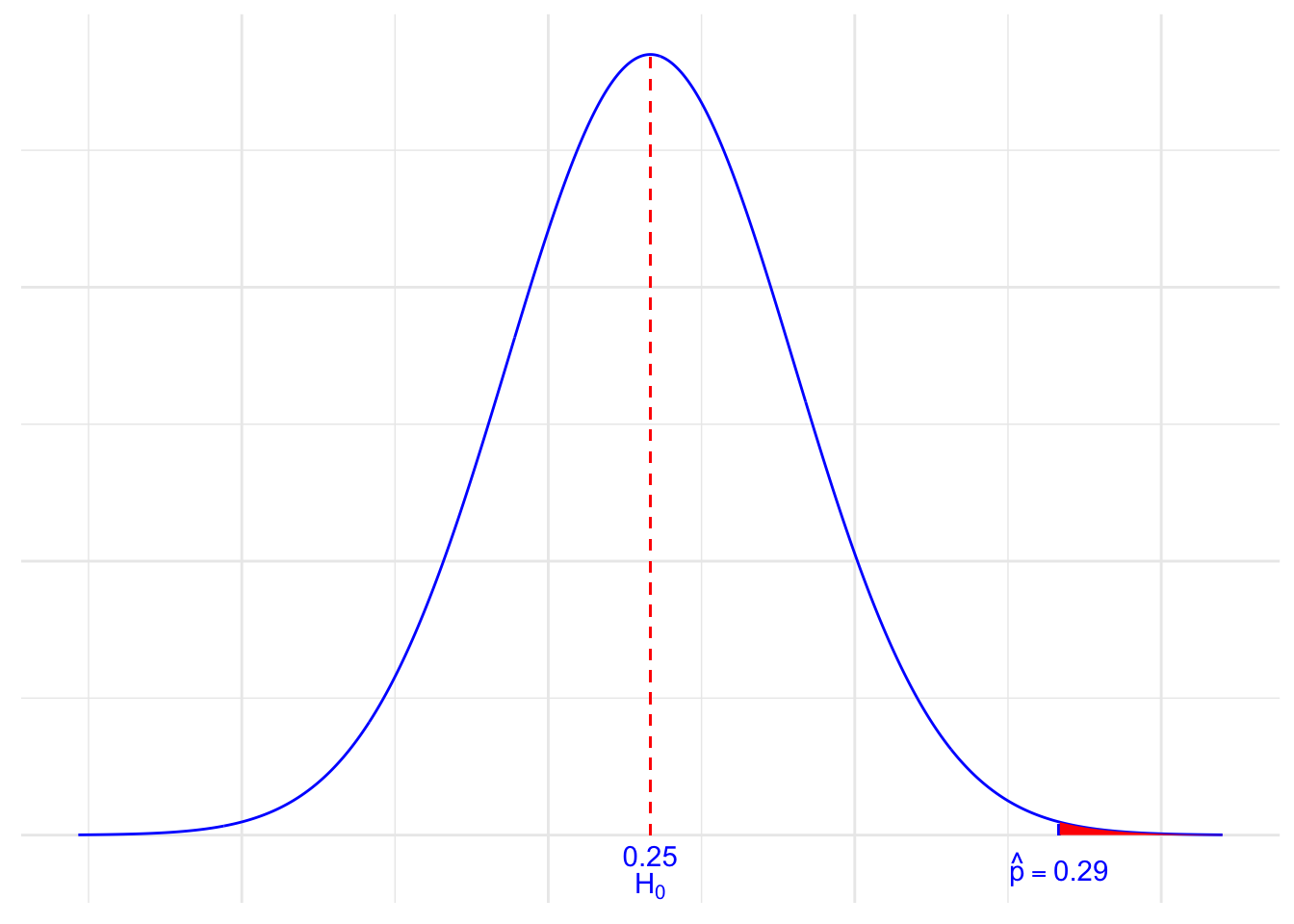
follows a standard normal \(N(0, 1)\) distribution. We can “translate” our observed sample proportion of 0.29 onto the \(Z\) scale. Here’s a picture that summarizes the situation:
So, we are assuming that the population proportion is 0.25, but we’ve observed a sample proportion of 0.290 that falls way out in the right tail of the normal distribution. It certainly doesn’t appear impossible to obtain a sample proportion of 0.29. But, that’s what we’re left with to decide. That is, we have to decide if a sample proportion of 0.290 is more extreme than we’d expect if the population proportion \(p\) does indeed equal 0.25.
The next step is to determine how to make a decision. There are two approaches to making the decision in hypothesis testing:
- One is called the “rejection region” (or critical value” or “critical region”) approach.
- The other is called the “p-value” approach.
First, let’s consider the rejection region approach.
Okay, so now let’s think about it. We probably wouldn’t reject our initial assumption that the population proportion \(p=0.25\) if our observed sample proportion were 0.255. And, we might still not be inclined to reject our initial assumption that the population proportion \(p=0.25\) if our observed sample proportion were 0.27. On the other hand, we would almost certainly want to reject our initial assumption that the population proportion \(p=0.25\) if our observed sample proportion were 0.35. That suggests, then, that there is some “threshold” value that once we “cross” the threshold value, we are inclined to reject our initial assumption. That is the critical value approach in a nutshell. That is, the critical value approach tells us to define a threshold value, called a “critical value” so that if our “test statistic” is more extreme than the critical value, then we reject the null hypothesis.
Recall that we set the significance level, \(\alpha\), as 5%. Since we are using the standard normal distribution, that would mean we would be looking for a \(Z\) value greater than 1.645. In other words, we decide to reject the null hypothesis \(H_0:p=0.25\) in favor of the “alternative hypothesis” \(H_a:p>0.25\) if:
\[Z>1.645 \text{ or equivalently } \hat{p}>0.273\]
Here’s a picture of such a “rejection region” (or “critical region”):
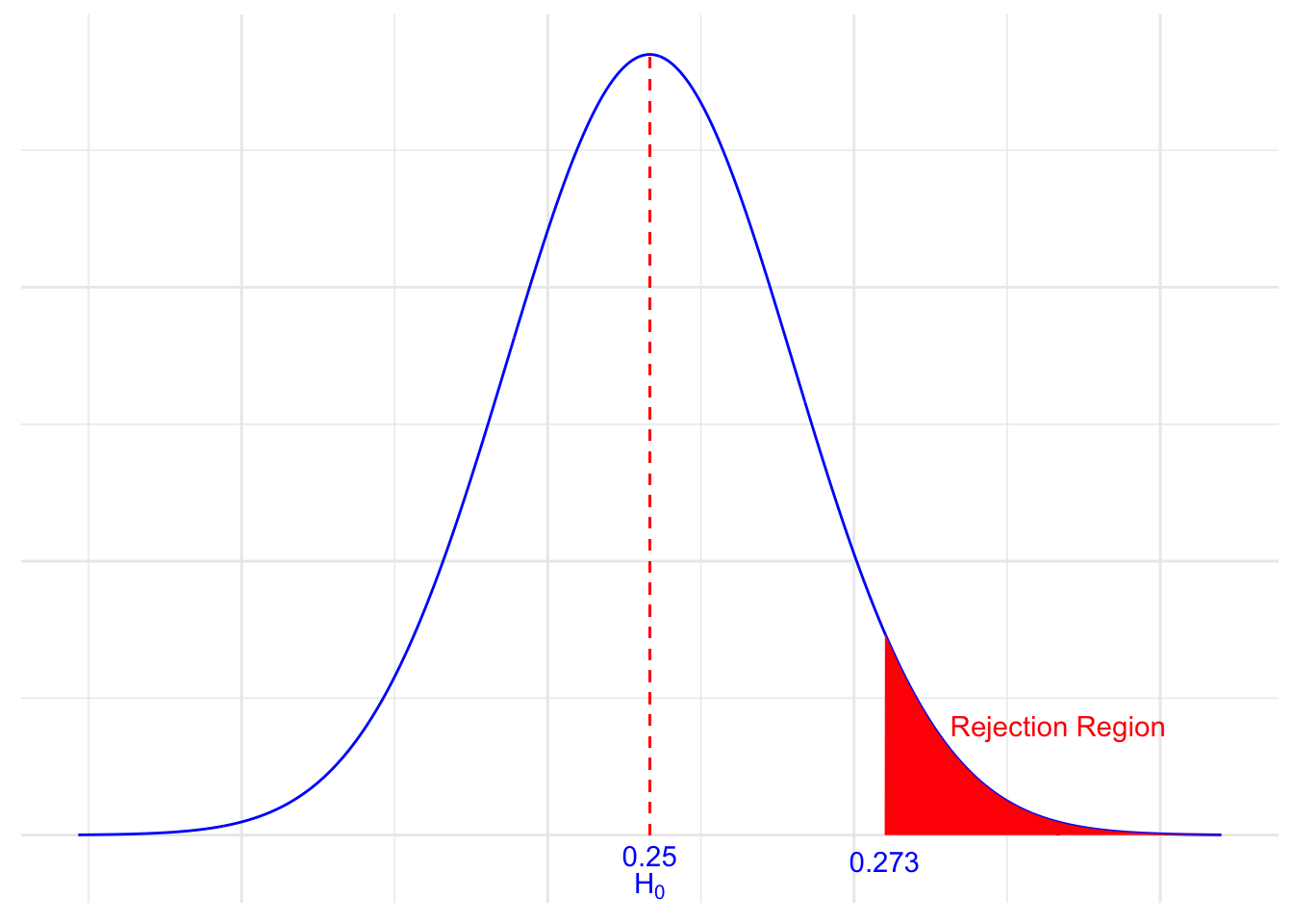
Note, by the way, that the “size” of the critical region is 0.05. This will become apparent in a bit when we talk below about the possible errors that we can make whenever we conduct a hypothesis test.
At any rate, let’s get back to deciding whether our particular sample proportion appears to be too extreme. Well, it looks like we should reject the null hypothesis (our initial assumption \(p=0.25\)) because:
\[\hat{p}=0.29>0.273\]
or equivalently since our test statistic:
\[Z=\dfrac{\hat{p}-p_0}{\sqrt{\dfrac{p_0(1-p_0)}{n}}}=\dfrac{0.29-0.25}{\sqrt{\dfrac{0.25(0.75)}{1000}}}=2.92\]
is greater than 1.645.
Our conclusion: we say there is sufficient evidence to conclude \(H_a:p>0.25\), that is, that the die is biased.
By the way, this example involves what is called a one-tailed test, or more specifically, a right-tailed test, because the critical region falls in only one of the two tails of the normal distribution, namely the right tail.
Before we continue on the next page looking at two more examples, let’s revisit the basic hypothesis testing procedure that we outlined above. This time, though, let’s state the procedure in terms of performing a hypothesis test for a population proportion using the critical value approach. The basic procedure is:
- State the null hypothesis \(H_0\) and the alternative hypothesis \(H_a\).
- Calculate the test statistic (found by using the distribution of the test, under the null hypothesis):
\[\begin{align*} Z=\dfrac{\hat{p}-p_0}{\sqrt{\dfrac{p_0(1-p_0)}{n}}} \end{align*}\]
- Determine the rejection region.
- Make a decision. Determine if the test statistic falls in the critical region. If it does, reject the null hypothesis. If it does not, do not reject the null hypothesis.
Now, back to those possible errors we can make when conducting such a hypothesis test.
9.3 Possible Errors
So, argh! Every time we conduct a hypothesis test, we have a chance of making an error. (Oh dear, why couldn’t I have chosen a different profession?!)
If we reject the null hypothesis \(H_0\) (in favor of the alternative hypothesis ) when the null hypothesis is in fact true, we say we’ve committed a Type I error. For our example above, we set P(Type I error) equal to 0.05:

Fig 9.3 We wanted to minimize our chance of making a Type I error! In general, we denote \(\alpha=P({\text{Type I error}})=\text{ the significance level}\). Obviously, we want to minimize \(\alpha\). Therefore, typical \(\alpha\) values are 0.01, 0.05, and 0.10.
If we fail to reject the null hypothesis when the null hypothesis is false, we say we’ve committed a Type II error. For our example, suppose (unknown to us) that the population proportion \(p\) is actually 0.27. Then, the probability of a Type II error, in this case, is:
\[\begin{align*} P(\text{Type II Error})=P(\hat{p}<0.273\quad if \quad p=0.27)=P\left(Z<\dfrac{0.273-0.27}{\sqrt{\dfrac{0.27(0.73)}{1000}}}\right)=P(Z<0.214)=0.5847 \end{align*}\]
In general, we denote \(\beta=P(\text{Type II error})\). Just as we want to minimize \(\alpha=P(\text{Type I error})\), we want to minimize \(\beta=P(\text{Type II error})\). Typical \(\beta\) values are 0.05, 0.10, and 0.20.
9.4 The p-value Approach
Up until now, we have used the critical region approach in conducting our hypothesis tests. Now, let’s take a look at an example in which we use what is called the P-value approach.
Example 9.4 (Lung Cancer) Part I
Among patients with lung cancer, usually, 90% or more die within three years. As a result of new forms of treatment, it is felt that this rate has been reduced. Let’s suppose in a recent study of n = 150 lung cancer patients, y = 128 died within three years. Is there sufficient evidence at the \(\alpha=0.05\) level, say, to conclude that the death rate due to lung cancer has been reduced?
Solution
The sample proportion is:
\[\begin{align*} \hat{p}=\dfrac{128}{150}=0.853 \end{align*}\]
The null and alternative hypotheses are: \[\begin{align*} H_0 \colon p = 0.90 \text { and } H_A: p<0.9 \end{align*}\]
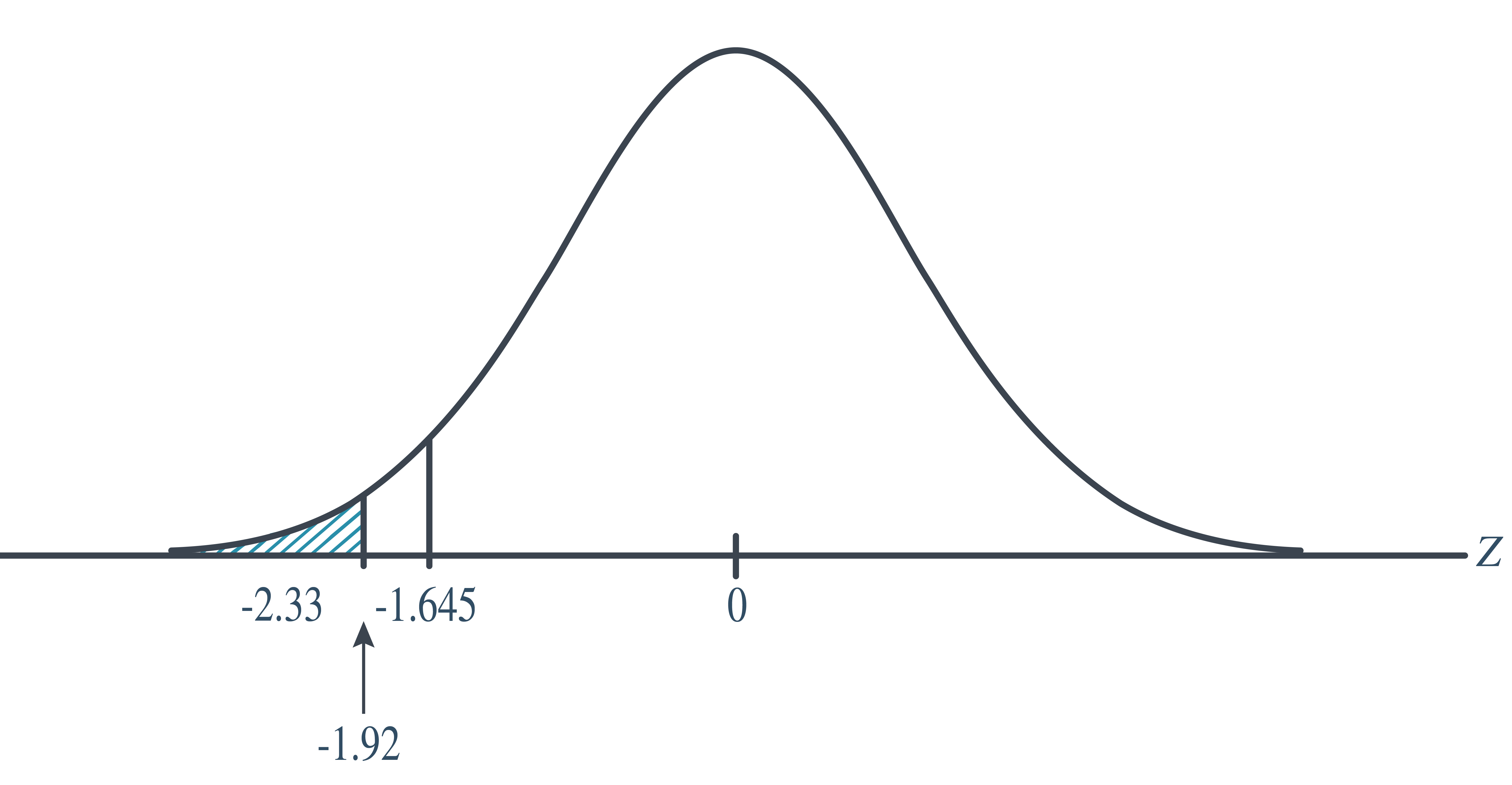
The test statistic is, therefore: \[\begin{align*} Z=\dfrac{\hat{p}-p_0}{\sqrt{\dfrac{p_0(1-p_0)}{n}}}=\dfrac{0.853-0.90}{\sqrt{\dfrac{0.90(0.10)}{150}}}=-1.92 \end{align*}\]
And, the rejection region is:
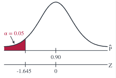
Since the test statistic \(Z = −1.92 < −1.645\), we reject the null hypothesis. There is sufficient evidence at the \(\alpha=0.05\) level to conclude that the rate has been reduced.
Part II
What if we set the significance level \(\alpha=P(\text{Type I error})=0.01\)? Is there still sufficient evidence to conclude that the death rate due to lung cancer has been reduced?
Solution
In this case, with \(\alpha=0.01\), the rejection region is \(Z ≤ −2.33\). That is, we reject if the test statistic falls in the rejection region defined by \(Z ≤ −2.33\):
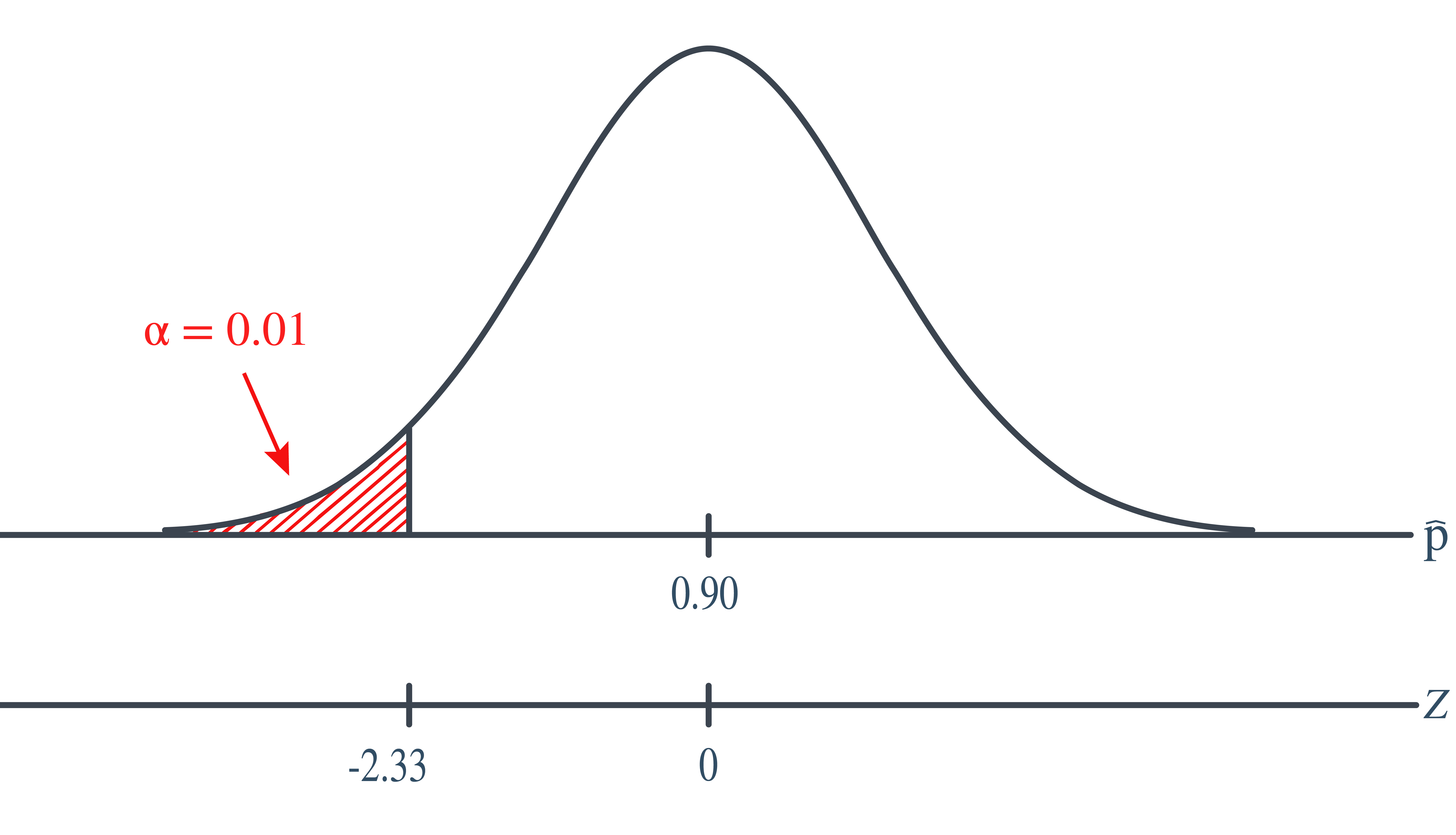
Because the test statistic \(Z = −1.92 > −2.33\), we do not reject the null hypothesis. There is insufficient evidence at the \(\alpha=0.01\) level to conclude that the rate has been reduced.
Part III
In the first part of this example, we rejected the null hypothesis when \(\alpha=0.05\). And, in the second part of this example, we failed to reject the null hypothesis when \(\alpha=0.01\). There must be some level of \(\alpha\), then, in which we cross the threshold from rejecting to not rejecting the null hypothesis. What is the smallest \(\alpha-\)level that would still cause us to reject the null hypothesis?
Solution
We would, of course, reject any time the critical value was smaller than our test statistic \(−1.92\):
That is, we would reject if the critical value were \(−1.645\), \(−1.83\), and \(−1.92\). But, we wouldn’t reject if the critical value were \(−1.93\). The \(\alpha-\)level associated with the test statistic \(−1.92\) is called the P-value. It is the smallest \(\alpha-\)level that would lead to rejection. In this case, the P-value is: \[\begin{align*} P(Z<-1.92)=0.0274 \end{align*}\]
Let’s formalize the definition of a P-value, as well as summarize the P-value approach to conducting a hypothesis test.
Def. 9.5 (P-value) The P-value is the smallest significance level that leads us to reject the null hypothesis.
Alternatively (and the way I prefer to think of P-values), the P-value is the probability that we’d observe a more extreme statistic than we did if the null hypothesis were true.
If the P-value is small, that is, if \(P\le \alpha\), then we reject the null hypothesis \(H_0\).
So far, all of the examples we’ve considered have involved a one-tailed hypothesis test in which the alternative hypothesis involved either a less than (\(<\)) or a greater than (\(>\)) sign. What happens if we aren’t sure of the direction in which the proportion could deviate from the hypothesized null value? That is, what if the alternative hypothesis involved a not-equal sign (\(\ne\))? Let’s take a look at an example.
Example 9.5 (Lung Cancer Continued) What if we wanted to perform a “two-tailed” test? That is, what if we wanted to test: \[\begin{align*} H_0: p=0.9 \text{ versus }H_a: p\ne 0.9 \end{align*}\] at the \(\alpha=0.05\) level?
Solution
Let’s first consider the critical value approach. If we allow for the possibility that the sample proportion could either prove to be too large or too small, then we need to specify a threshold value, that is, a critical value, in each tail of the distribution. In this case, we divide the “significance level” \(\alpha\) by 2 to get \(\frac{\alpha}{2}\):
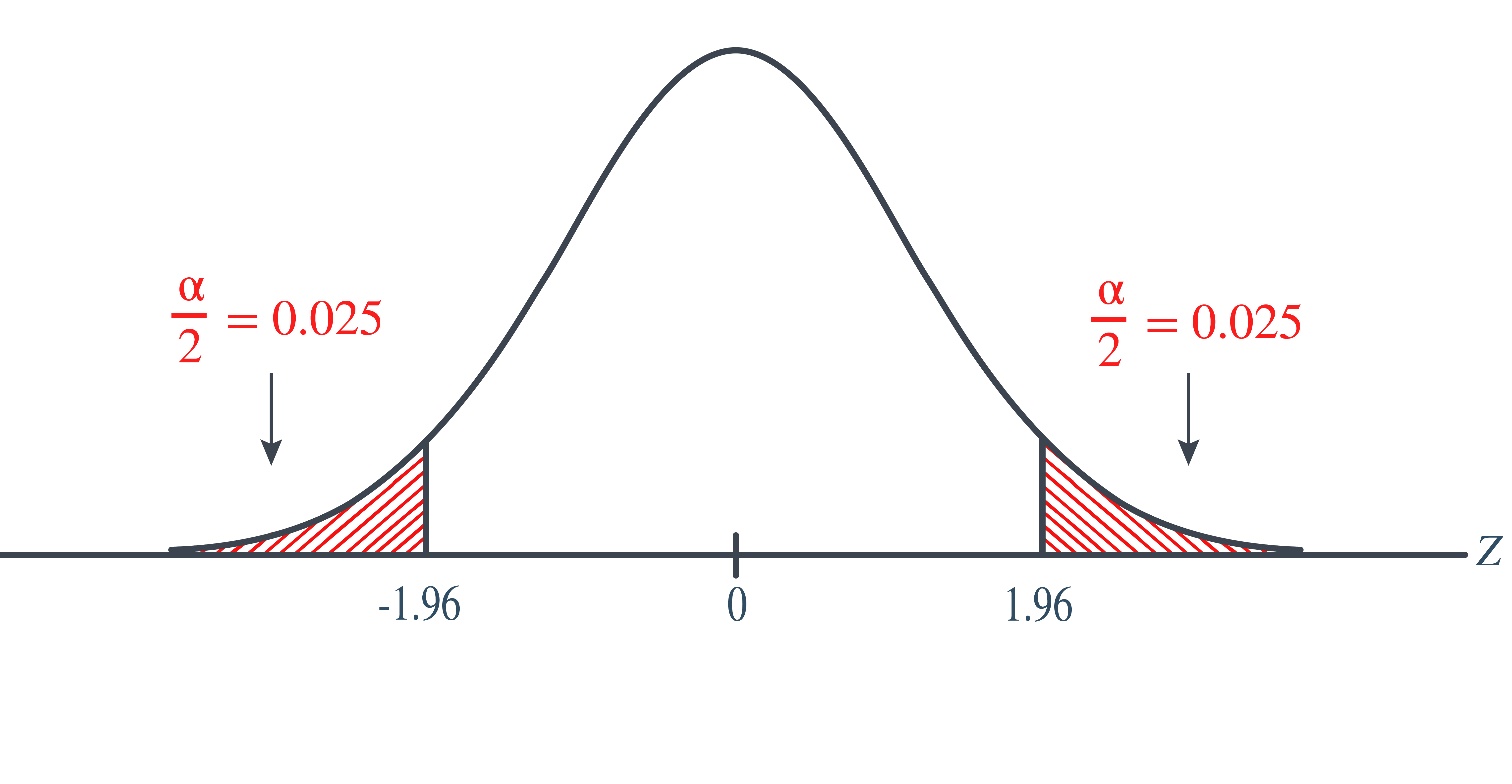
That is, our rejection rule is that we should reject the null hypothesis or we should reject the null hypothesis \(H_0\). Alternatively, we can write that we should reject the null hypothesis \(H_0\) if \(|Z|\ge 1.96\). Because our test statistic is \(−1.92\), we just barely fail to reject the null hypothesis, because \(1.92 < 1.96\). In this case, we would say that there is insufficient evidence at the \(\alpha=0.05\) level to conclude that the sample proportion differs significantly from 0.90.
Now for the P-value approach. Again, needing to allow for the possibility that the sample proportion is either too large or too small, we multiply the P-value we obtain for the one-tailed test by 2:
That is, the P-value is:
\[\begin{align*} P=P(|Z|\geq 1.92)=P(Z>1.92 \text{ or } Z<-1.92)=2 \times 0.0274=0.055 \end{align*}\]
Because the P-value 0.055 is (just barely) greater than the significance level \(\alpha=0.05\), we barely fail to reject the null hypothesis. Again, we would say that there is insufficient evidence at the \(\alpha=0.05\) level to conclude that the sample proportion differs significantly from 0.90.
9.5 Tests about One Mean
In this lesson, we will continue our investigation of hypothesis testing. We will focus our attention on hypothesis tests for a population mean, \(\mu\), under different situations.
Variance Known
Let’s start by acknowledging that it is completely unrealistic to think that we’d find ourselves in the situation of knowing the population variance, but not the population mean. Therefore, the hypothesis testing method that we learn on this page has limited practical use. We study it only because we’ll use it later to learn about the “power” of a hypothesis test (by learning how to calculate Type II error rates). As usual, let’s start with an example.
Example 9.6 Boys of a certain age are known to have a mean weight of \(\mu=85\) pounds. A complaint is made that the boys living in a municipal children’s home are underfed. As one bit of evidence, \(n=25\) boys (of the same age) are weighed and found to have a mean weight of \(\bar{x} = 80.94\) pounds. It is known that the population standard deviation \(\sigma\) is 11.6 pounds (the unrealistic part of this example!). Based on the available data, what should be concluded concerning the complaint?
Solution
The null hypothesis is \(H_0:\mu=85\), and the alternative hypothesis is \(H_a:\mu<85\). In general, we know that if the weights are normally distributed, then:
\[\begin{align*} Z=\dfrac{\bar{X}-\mu}{\sigma/\sqrt{n}} \end{align*}\]
follows the standard normal \(N(0,1)\) distribution. It is actually a bit irrelevant here whether or not the weights are normally distributed, because the same size \(n=25\) is large enough for the Central Limit Theorem to apply. In that case, we know that \(Z\), as defined above, follows at least approximately the standard normal distribution. At any rate, it seems reasonable to use the test statistic:
\[\begin{align*} Z=\dfrac{\bar{X}-\mu_0}{\sigma/\sqrt{n}} \end{align*}\]
for testing the null hypothesis
\[\begin{align*} H_0:\mu=\mu_0 \end{align*}\]
against any of the possible alternative hypotheses \(H_a: \mu\ne\mu_0\), \(H_a:\mu<\mu_0\), and \(H_a:\mu>\mu_0\).
For the example in hand, the value of the test statistic is:
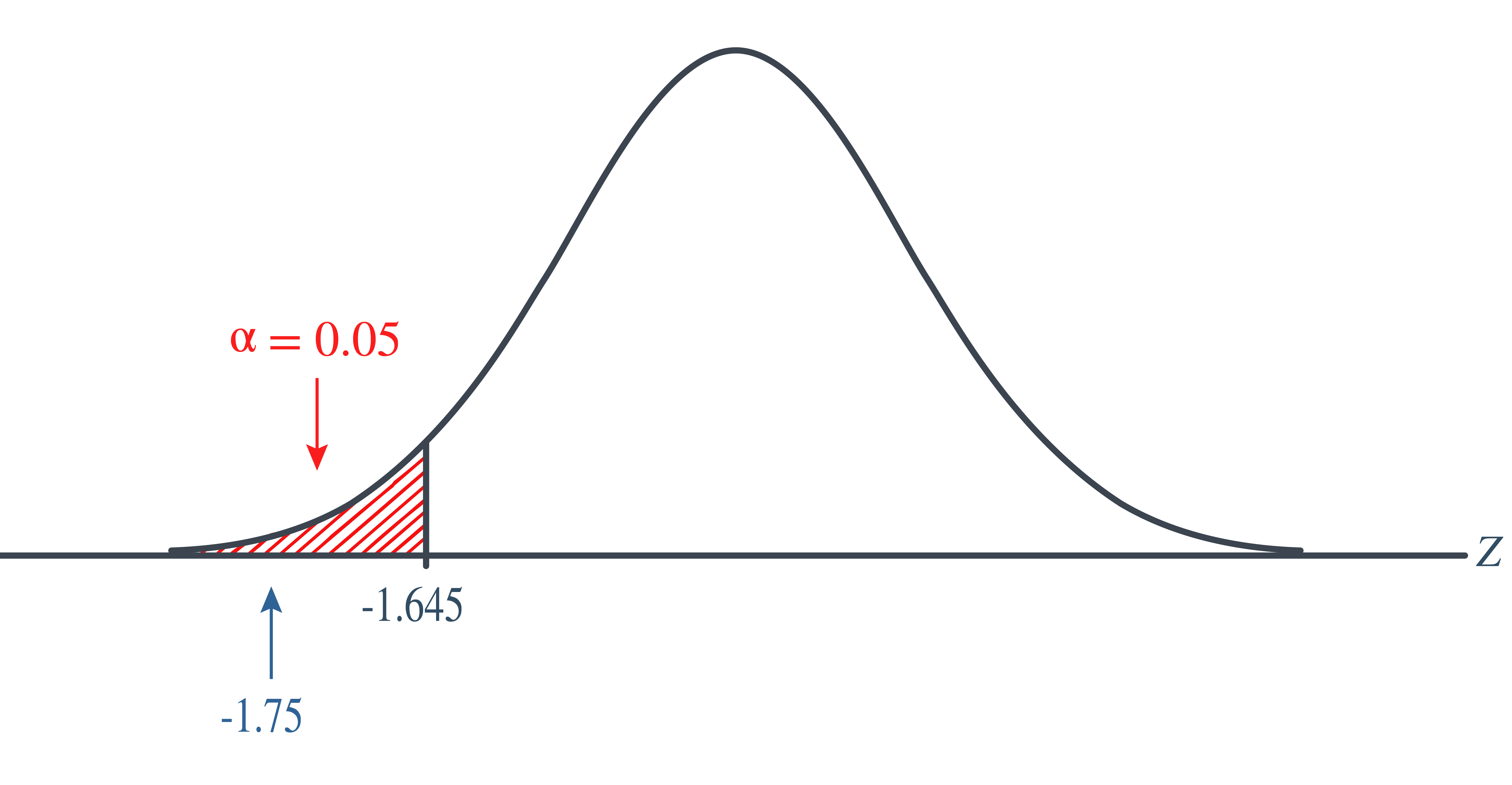
\[\begin{align*} Z=\dfrac{80.94-85}{11.6/\sqrt{25}}=-1.75 \end{align*}\]
The critical region approach tells us to reject the null hypothesis at the \(\alpha=0.05\) level if \(Z<-1.645\). Therefore, we reject the null hypothesis because \(Z=-1.75<-1.645\), and therefore falls in the rejection region:
As always, we draw the same conclusion by using the \(p\)-value approach. Recall that the \(p\)-value approach tells us to reject the null hypothesis at the \(\alpha=0.05\) level if the \(p\)-value\(\le \alpha=0.05\). In this case, the \(p\)-value is \(P(Z<-1.75)=0.0401\):
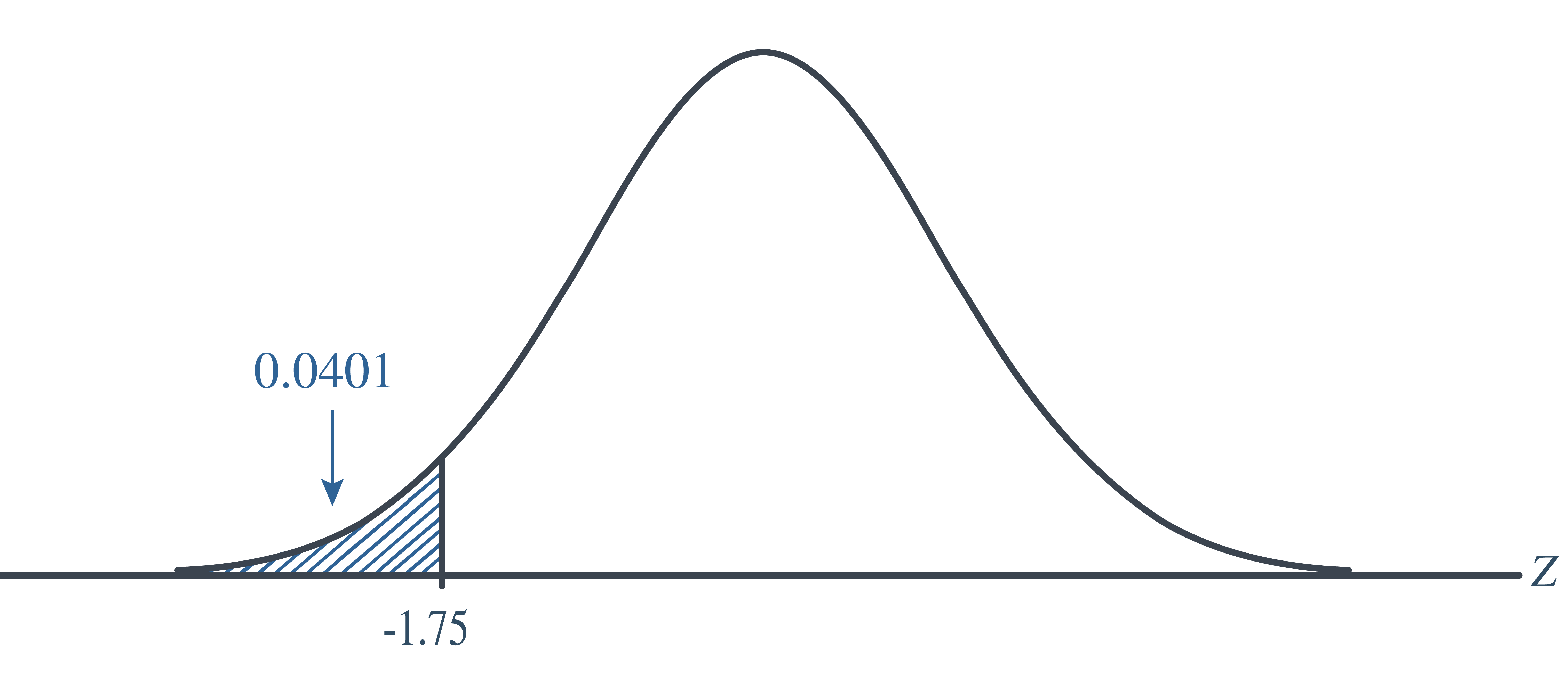
As expected, we reject the null hypothesis because the \(p\)-value\(=0.401<\alpha=0.05\).
Variance Unknown
Now that, for purely pedagogical reasons, we have the unrealistic situation (of a known population variance) behind us, let’s turn our attention to the realistic situation in which both the population mean and population variance are unknown.
Example 9.7 It is assumed that the mean systolic blood pressure is \(\mu=120\)mm Hg. In the Honolulu Heart Study, a sample of \(n=100\) people had an average systolic blood pressure of 130.1 mm Hg with a standard deviation of 21.21 mm Hg. Is the group significantly different (with respect to systolic blood pressure!) from the regular population?
Solution
The null hypothesis is \(H_0:\mu=120\), and because there is no specific direction implied, the alternative hypothesis is \(H_a: \mu\ne 120\).
The next step for hypothesis testing is to determine the significance level, or the probability of a Type I error. For this example, let us set \(\alpha=0.05\).
Step 3 is to calculate the test statistic. Recall that we should determine a test statistic with a known distribution, under the assumptions and the null hypothesis. From STAT 414, we know that if the data are normally distributed, then:
\[\begin{align*} T=\dfrac{\bar{X}-\mu}{S/\sqrt{n}} \end{align*}\]
follows a \(t\)-distribution with \(n-1\) degrees of freedom. Therefore, it seems reasonable to use the test statistic:
\[\begin{align*} T=\dfrac{\bar{X}-\mu_0}{S/\sqrt{n}} \end{align*}\]
for testing the null hypothesis \(H_0:\mu=120\) against any of the possible alternative hypotheses \(H_a:\mu\ne\mu_0\), \(H_a:\mu<\mu_0\), and \(H_a:\mu>\mu_0\). For the example in hand, the value of the test statistic is:
\[\begin{align*} t=\dfrac{130.1-120}{21.21/\sqrt{100}}=4.762 \end{align*}\]
The critical region approach tells us to reject the null hypothesis at the \(\alpha=0.05\) level if \(t\ge t_{0.025, 99}=1.9842\) or if \(t\le t_{0.025, 99}=-1.9842\). Therefore, we reject the null hypothesis because \(t=4.762>1.9842\), and therefore falls in the rejection region:
Again, as always, we draw the same conclusion by using the \(p\)-value approach. The \(p\)-value approach tells us to reject the null hypothesis at the \(\alpha=0.05\) level if the \(p\)-value\(\le 0.05\). In this case, the \(p\)-value is:
\[\begin{align*} 2P(T_{99}>4.762)<2P(T_{99}>1.9842)=2(0.025)=0.05 \end{align*}\]
As expected, we reject the null hypothesis because \(p\)-value\(\le 0.01<\alpha=0.05\).
9.6 Summary
In this lesson, we introduced the framework of hypothesis testing—a formal way to use sample data to evaluate claims about a population parameter. The big idea is to set up two competing statements: the null hypothesis (\(H_0\)), which represents the status quo or no effect, and the alternative hypothesis (\(H_a\)), which represents what we’re trying to find evidence for.
We compute a test statistic, which summarizes the evidence from the sample, and determine how extreme it is under the assumption that \(H_0\) is true. This leads us to a rejection region or a p-value approach. If our test statistic falls in the rejection region or if the p-value is smaller than the significance level \(\alpha\), we reject \(H_0\).
Key Takeaways:
- A typical form of a test statistic is: \(Z=\frac{\hat{\theta}-\theta_0}{SE(\hat{\theta})}\)
- Type I error: rejecting when it’s actually true, \(P(\text{Type I error})=\alpha\)
- Type II error: failing to reject when is true, \(P(\text{Type II error})=\beta\)
- The power of a test is the probability of correctly rejecting \(H_0\): \(\text{Power}=1-\beta\)
We also defined two types of errors: - Type I error: rejecting \(H_0\) when it’s actually true (probability \(\alpha\)) - Type II error: failing to reject \(H_0\) when \(H_a\) is true (probability \(\beta\))
The power of a test is the probability of correctly rejecting \(H_0\):
\[ \text{Power} = 1 - \beta \]