6 Confidence Intervals
In this lesson, we are going to take a brief break from MLEs. Don’t worry! We will go back to maximum likelihood estimation.
In this lesson, we’ll learn how to construct and calculate a confidence interval for a population parameter. As we’ll soon see, a confidence interval is an interval (or range) of values that we can be really confident contains the true unknown population parameter. We’ll spend some time working on understanding the “confidence part” of an interval, as well as learning what factors affect the length of an interval.
Objectives
Upon completion of this lesson, you should be able to:
- Be able to correctly interpret a given confidence interval in terms of the population,
- Analytically construct a confidence interval for an unknown parameter, and
- Numerically calculate a confidence interval for an unknown parameter given a set of data.
6.1 Introduction to Confidence Intervals
So far, when we discuss estimation, we have focused on finding an estimator, or point estimate, for a parameter. In this section, we will introduce interval estimates.
When we use the sample mean \(\bar{x}\) to estimate the population mean \(\mu\), can we be confident that \(\bar{x}\) is close to \(\mu\)? And, when we use the sample proportion \(\hat{p}\) to estimate the population proportion \(p\), can we be confident that \(\hat{p}\) is close to \(p\)?
Do we have any idea as to how close the sample statistic is to the population parameter?
Rather than using just a point estimate, we could find an interval (or range) of values that we can be really confident contains the actual unknown population parameter. For example, we could find lower ( \(L\) ) and upper ( \(U\) ) values between which we can be really confident the population parameter, \(\theta\), falls:
\[L< \theta<U\]
An interval of such values is called a confidence interval. Each interval has a confidence coefficient (reported as a proportion):
\[1-\alpha\]
or a confidence level (reported as a percentage):
\[(1-\alpha)100\%\]
Typical confidence coefficients are 0.90, 0.95, and 0.99, with corresponding confidence levels of 90%, 95%, and 99%. For example, upon calculating a confidence interval for a parameter \(\theta\) with a confidence level of, say 95%, we can say:
“We can be 95% confident that the population parameter falls between \(L\) and \(U.\)”
As should agree with our intuition, the greater the confidence level, the more confident we can be that the confidence interval contains the actual population parameter.
6.2 Population Mean of a Normal Distribution
Let’s demonstrate how to construct an interval estimate (or confidence interval) for the population mean of the Normal distribution with known variance \(\sigma^2.\)
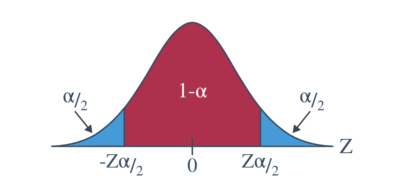
Before we do, we should define our notation. Recall the value \(z_{\alpha/2}\) is the \(Z\) value (obtained from a standard normal table) such that the area to the right of it under the standard normal curve is \(\frac{\alpha}{2}.\) That is:
\[P(Z\ge z_{\alpha/2})=\alpha/2\]
Likewise:
\[-z_{\alpha/2}\]
is the \(Z\)-value (obtained from a standard normal table) such that the area to the left of it under the standard normal curve is \(\frac{\alpha}{2}.\) That is:
\[P(Z\le -z_{\alpha/2})=\alpha/2\]
I like to illustrate this notation with the following diagram of a standard normal curve:
With the notation now recalled, let’s state the formula for a confidence interval for the population mean.
6.3 Interpretation
The topic of interpreting confidence intervals is one that can get frequentist statisticians all hot under the collar. Let’s try to understand why!
Although the derivation of the \(Z\)-interval for a mean technically ends with the following probability statement:
\[P\left[\bar{X}-z_{\alpha/2}\frac{\sigma}{\sqrt{n}}\le \mu\le \bar{X}+z_{\alpha/2}\frac{\sigma}{\sqrt{n}} \right]=1-\alpha\]
it is incorrect to say:
“The probability that the population mean \(\mu\) falls between the lower value \(L\) and the upper value \(U\) is \(1-\alpha.\)”
But why? Probability statements are about random variables. The population mean \(\mu\) is a constant, not a random variable. It makes no sense to make a probability statement about a constant that does not change.
So, in short, frequentist statisticians don’t like to hear people trying to make probability statements about constants, when they should only be making probability statements about random variables. So, okay, if it’s incorrect to make the statement that seems obvious to make based on the above probability statement, what is the correct understanding of confidence intervals? Here’s how frequentist statisticians would like the world to think about confidence intervals:
Suppose we take a large number of samples, say 1000.
Then, we calculate a 95% confidence interval for each sample.
Then, “95% confident” means that we’d expect 95%, or 950, of the 1000 intervals to be correct, that is, to contain the actual unknown value \(\mu.\)
So, what does this all mean in practice?
In reality, we take just one random sample. The interval we obtain is either correct or incorrect. That is, the interval we obtain based on the sample we’ve taken either contains the true population parameter or it does not. Since we don’t know the value of the true population parameter, we’ll never know for sure whether our interval is correct or not. We can just be very confident that we obtained a correct interval (because 95% of the intervals we could have obtained are correct).
Example 6.1 Let’s consider another example where we may have to recall some of the material learned in STAT 414.
Let \(Y\) be a a random variable with a Gamma distribution with known parameter \(\alpha=2\) and unknown parameter, \(\theta.\) We want to construct a 90% confidence interval for \(\theta.\)
For us to do this, we need to find a pivotal quantity. A pivotal quantity poses two characteristics:
- It is a function of the sample measurements and the only unknown parameter, \(\theta.\)
- The distribution of the pivotal quantity does not depend on \(\theta.\)
Therefore, we must construct a function of \(Y\) and \(\theta\) that has a distribution that does not depend on \(\theta.\) Thus, we need to find a pivotal quantity. It is helpful to recall distributions of functions of random variables back from STAT 414.
Consider the quantity \(U=\frac{2Y}{\theta}.\) What is the distribution of \(U\)? Let’s use the moment generating function method we get the distribution of \(U.\)
\[\begin{align*} &M_Y(t)=E(e^{tY})=\frac{1}{(1-\theta t)^2}\\ &M_U(t)=E(e^{tU})=E(e^{t\left(\frac{2Y}{\theta}\right)})=E(e^{\left(\frac{2t}{\theta}\right)Y})=\frac{1}{\left(1-\theta\left(\frac{2t}{\theta}\right)\right)^2}=\frac{1}{(1-2t)^2} \end{align*}\]
Due to the uniqueness property of the moment generating function, we can see that \(U\) is a Gamma distribution with parameters \(\alpha=2\) and \(\theta=2.\) Even more useful, we can see that \(U\) follows a chi-square distribution with \(r=4\) degrees of freedom. It is very useful to view the distribution as a chi-square because we have software and also tables to help us find the probabilities.
Now, lets construct the confidence interval.
We want the interval such that:
\[P\left[\chi^2_{0.05}(4)\le \frac{2Y}{\theta}\le \chi^2_{0.95}(4)\right]=1-\alpha\]
Again, we only consider the expression in the brackets, we get:
\[\frac{1}{\chi^2_{0.95}(4)}\le \frac{\theta}{2Y}\le \frac{1}{\chi^2_{0.05}(4)}\]
\[\frac{2Y}{\chi^2_{0.95}(4)}\le \theta \le \frac{2Y}{\chi^2_{0.05}(4)}\]
Therefore, the 90% confidence interval for \(\theta\) is:
\[\left[\frac{2Y}{\chi^2_{0.95}(4)}, \frac{2Y}{\chi^2_{0.05}(4)}\right]\]
Finally, let’s find the confidence interval with some data. Suppose we have an observation of \(y=1.261552\) from a Gamma distribution with parameters \(\alpha=2\) and \(\theta.\) Let’s find and interpret a 90% confidence interval for \(\theta.\)
\[\left[\frac{2(1.261552)}{9.4877}, \frac{2(1.261552)}{0.7107}\right]=\left[0.2659, 3.5502\right]\]
We are 90% confident that the true value of \(\theta\) is between 0.2659 and 3.5502.
The biggest challenge in constructing the confidence interval is finding the pivotal quantity. In the examples we have in this class, the pivotal quantity will be provided or there will be some direction to lead you to finding the pivotal quantity. Don’t worry, we will have plenty of practice constructing confidence intervals from the homework.
6.4 Large Sample Confidence Intervals
Suppose we have an unbiased estimator, \(\hat{\theta}\), with standard error \(\sigma_{\hat{\theta}}\) . Under certain conditions (will discuss later), for large samples:
\[Z=\frac{\hat{\theta}-\theta}{\sigma_{\hat{\theta}}}\]
follows an approximately standard normal distribution. Additionally, \(Z=\frac{\hat{\theta}-\theta}{\sigma_{\hat{\theta}}}\), forms (approximately) a pivotal quantity that can be used to construct a confidence interval for the unknown parameter, \(\theta.\)
The conditions are:
- The expected value of the estimator, \(\hat{\theta}\) , should be \(\theta.\) In other words, the estimator needs to be unbiased.
- The standard error of the estimator, \(\sigma_{\hat{\theta}}\) , is known or can be found.
- The distribution of the estimator possesses a distribution that is approximately normal for large samples. One example is the Central Limit Theorem.
Example 6.2 The shopping times of \(n=64\) randomly selected customers at a local supermarket were recorded. The average and variance of the 64 shopping times were 33 minutes and 256 \(\text{minutes}^2\), respectively. Estimate the true mean shopping time per customer with 0.9 confidence.
Solution
The confidence interval would take the form of:
\[\hat{\theta}\pm z_{\alpha/2}\sigma_{\hat{\theta}}\]
We want to estimate the population mean shopping time, \(\mu.\) We have an estimate of \(\mu\), namely \(\hat{\mu}=33.\) The estimated standard error of the estimator is \(\hat{\sigma}^2_{\hat{\mu}}=\frac{s}{\sqrt{64}}=256.\) The interval would be:
\[\hat{\mu}\pm z_{\alpha/2}\left(\hat{\sigma}_{\hat{\mu}}\right)=\left(33\pm 1.645\left(\frac{16}{8}\right)\right)=(29.71, 36.29)\]
6.5 Summary
In this lesson, we shifted from point estimates to something even more informative—confidence intervals. Instead of just giving a single number as an estimate (like the sample mean), we now give a range of values that we believe, with a certain level of confidence, contains the true population parameter.
We spent time unpacking what that confidence level actually means. A 95% confidence interval doesn’t mean there’s a 95% chance the parameter is in the interval you got—because the parameter is fixed. What it does mean is that if we repeated this process over and over, 95% of those intervals would contain the true value.
You learned how to construct these intervals using known distributions, pivotal quantities, and large-sample approximations.
The big picture? Confidence intervals help us communicate uncertainty in a clear, honest way, and they’re a key tool in the statistician’s toolkit.
Key Takeaways:
- A general form of a confidence interval is: \(\text{Point Estimate }\pm \text{(Critical Value)}\times \text{Standard Error}\)
- The confidence interval ror a population mean when the variance is known for a Normal distribution: \(\bar{X}\pm z_{\alpha/2}\cdot \frac{\sigma}{\sqrt{n}}\)
- The confidence interval for a population mean of a Normal distribution when the variance is unknown: \(\bar{X}\pm t_{\alpha/2, df}\cdot \frac{s}{\sqrt{n}}\)
- Sample size, confidence level, and variability affect the width of an interval.