2 Estimation (Part I)
Point Estimation
Unbiased Estimation
Bias
Variance and Mean Square
Factorization
Sufficiency
Method of Moments
This lesson introduces the fundamental concepts of point estimation, a cornerstone of statistical inference. You will learn how to estimate unknown population parameters, such as means and proportions, using sample data. Through this lesson, you will develop the skills to compute maximum likelihood estimates for various single-parameter models and evaluate the quality of estimators using key properties such as bias, variance, and mean square error. Practical examples, including estimating health insurance coverage among college students and analyzing COVID-19 death rates, will illustrate these concepts. By the end of this lesson, you will have a robust understanding of point estimation and be well-prepared for advanced topics in statistical estimation.
Objectives
Upon completion of this lesson, you should be able to:
- Determine the distribution of estimators,
- Calculate and interpret the bias of an estimator,
- Calculate the variance and mean squared error of an estimator, and
- Use estimator properties to compare and identify those that are better under certain criteria.
2.1 Point Estimation
Suppose we have an unknown population parameter, such as a population mean \(\mu\) or a population proportion \(p\), which we’d like to estimate. For example, suppose we are interested in estimating:
- \(p\) = the (unknown) proportion of American college students, 18-24, who have health insurance
- \(\mu\) = the (unknown) mean number of days it takes Alzheimer’s patients to achieve certain milestones
In either case, we can’t possibly survey the entire population. That is, we can’t survey all American college students between the ages of 18 and 24. Nor can we survey all patients with Alzheimer’s disease. So, of course, we do what comes naturally and take a random sample from the population, and use the resulting data to estimate the value of the population parameter. Of course, we want the estimate to be “good” in some way.
We’ll also learn ways of assessing whether a point estimate is “good.” We’ll do that by defining what it means for an estimate to be unbiased, defining what it means to be sufficient, finding the variance of the estimate, and the mean square error.
Definitions and Notation
We’ll start the lesson with some formal definitions. In doing so, recall that we denote the \(n\) random variables arising from a random sample as subscripted uppercase letters:
\[X_1, X_2, \ldots, X_n\]
The corresponding observed values of a specific random sample are then denoted as subscripted lowercase letters:
\[x_1, x_2, \ldots, x_n\]
Def. 2.1 (Parameter Space) The range of possible values of the parameter \(\theta\) is called the parameter space \(\Omega\) (the Greek letter “omega”).
Example 2.1 If \(\mu\) denotes the mean grade point average of all college students, then the parameter space (assuming a 4-point grading scale):
\[\Omega = \{\mu: 0 \le \mu \le 4\}\]
If \(p\) is the proportion of students who smoke cigarettes, then the parameter space is:
\[\Omega = \{p: 0 \le p \le 1\}\]
2.1.1 Point Estimator
The function \(X_1, X_2, \ldots X_n\), that is, the statistic \(u(X_1, X_2, \ldots, X_n)\), used to estimate \(\theta\) is called a point estimator of \(\theta.\)
Example 2.2 For example, the function:
\[\bar{X} = \frac{1}{n} \sum_{i=1}^n X_i\] is a point estimator of the population mean \(\mu.\)
When \(X_i = 0\) or 1, the function:
\[\hat{p} = \frac{1}{n} \sum_{i=1}^n X_i\]
is a point estimator of the population proportion \(p.\)
The function:
\[S^2 = \frac{1}{n-1} \sum_{i=1}^n (X_i - \bar{X})^2\]
is a point estimator of the population variance \(\sigma^2.\)
2.1.2 Point Estimate
The function \(u(x_1, x_2, \ldots, x_n)\) computed from a set of data is an observed point estimate of \(\theta.\)
Example 2.3 If \(x_i\), \(i = 1, \ldots, 88\) are the observed grade point averages of a sample of 88 students, then,
\[\bar{x} = \frac{1}{88} \sum_{i=1}^{88} x_i = 3.12\] is a point estimate of \(\mu\), the mean grade point average of all students in the population.
Recall the probability density function (or the probability mass function) of a random variable has been defined as \(f(x).\) We define a probability model for the data as:
\[x_i \sim f_x(x_i|\theta)\]
where \(f_x\) is the probability distribution and \(\theta\) is the parameter (or parameters) in the model.
If \(\theta\) is known, our work is done. The goal of this course is to understand what to do when \(\theta\) is not known. We define the estimator of \(\theta\) as \(\hat{\theta}.\) \(\hat{\theta}\) is a function of our data, i.e. \(\hat{\theta} = g(X_1, X_2, \ldots, X_n).\) We will use this function of data to help us understand \(\theta.\) We will be performing statistical inference. Statistical Inference is using data to infer properties of an underlying distribution.
Let’s go through a motivational example that uses some of these terms and shows where we are going.
Example 2.4 Suppose a researcher is interested in COVID-19. Let - \(n_{c,y} =\) number of people with COVID in country \(c\) and in year \(y\) - \(d_{c,y} =\) number of people who died of COVID in country \(c\) and in year \(y\)
For example, \(n_{\text{USA}, 2021}\) is the number of people with COVID in the United States of America in the year 2021.
Suppose we want to answer if COVID-19 death rates are lower in 2022 (after the vaccine) than in 2021 (before the vaccine) for a particular country. We need to define a probability model for \((n_{c,y}, d_{c,y}).\) Suppose the model is:
\[d_{c,y} \sim \text{Bin}(n_{c,y}, p_y)\]
In this model, the parameter is \(p_y\), the probability of a COVID death in year \(y.\) Since we are interested in comparing 2022 and 2021, we have two parameters, \(p_{2021}\) and \(p_{2022}.\) If we knew the parameters, we would answer the question. Since we do not, we need to estimate \(\theta = (p_{2021}, p_{2022}).\)
Now what? What is \(\hat{\theta}\)? How do we determine the estimator? Could there be more than one estimator? We will learn how to find an estimator of unknown parameters in a little while. For now, we will find out how to compare estimators.
2.2 Properties of Estimators
Suppose we are given multiple estimators of an unknown parameter, \(\theta.\) How do we know which is the “better” choice? Consider the following example.
Example 2.5 Suppose we have an independent and identically distributed (i.i.d) sample of size \(n=3\) such that
\[X_i \overset{iid}{\sim} \text{Bin}(10, p)\]
The unknown parameter in this case is \(p\), the probability of a success. Define three possible estimators of \(p\) as:
\[\begin{aligned} \hat{p}_1 = \frac{X_1}{n} \\ \hat{p}_2 = \frac{\frac{X_1}{10} + \frac{X_2}{10} + \frac{X_3}{10}}{3} = \frac{X_1 + X_2 + X_3}{30} \\ \hat{p}_3 = \hat{p}_2 + 0.1 = \frac{X_1 + X_2 + X_3}{30} + 0.1 \end{aligned}\]
Which estimator does a better job estimating \(p\)? We can start by defining the bias of an estimate.
Def. 2.2 (Unbiased Estimation) One measure of a “good” estimator is “unbiasedness.” An estimator is said to be unbiased if the expected value of the estimator is the unknown parameter \(\theta.\)
2.2.1 Bias
If the following holds:
\[E\left[u(X_1, X_2, \ldots, X_n)\right] = \theta\]
then the statistic \(u(X_1, X_2, \ldots, X_n)\) is an unbiased estimator of the parameter \(\theta.\) Otherwise, \(u(X_1, X_2, \ldots, X_n)\) is a biased estimator of \(\theta.\) The bias of the statistic is defined as:
\[\text{Bias} = E(u(X_1, X_2, \ldots, X_n)) - \theta\] Note that an unbiased estimator will have a bias of \(\text{Bias} = E(u(X_1, X_2, \ldots, X_n)) - \theta = 0.\)
Example 2.6 Consider the previous example where we define our estimators of \(p\) as:
\[\begin{aligned} & \hat{p}_1 = \frac{X_1}{10} \\ & \hat{p}_2 = \frac{X_1 + X_2 + X_3}{30} \\ & \hat{p}_3 = \hat{p}_2 + 0.1 = \frac{X_1 + X_2 + X_3}{30} + 0.1 \end{aligned}\]
What is the bias of the estimators?
Solution
To find the bias of each estimator, we need to find their expected values. Recall for a Binomial random variable, \(X\), we know \(E(X) = p\) and \(\text{Var}(X) = np(1-p).\) Let’s start with \(\hat{p}_1.\)
\[\begin{align}\text{Bias}_1 &= E(\hat{p}_1) - p\\ &= E\left[\frac{X_1}{10}\right] - p\\ &= \frac{E(X_1)}{10} - p\\ &= \frac{10p}{10} - p\\ &= p - p = 0 \end{align}\]
Example 2.7 If \(X_i\) are normally distributed random variables with mean \(\mu\) and variance \(\sigma^2\), then consider the two estimators of \(\mu\) and \(\sigma^2\), respectively:
\[\begin{align*} \hat{\mu} &= \frac{1}{n}\sum_{i=1}^n X_i, \\ \quad \hat{\sigma}^2 &= \frac{\sum_{i=1}^n(X_i - \bar{X})^2}{n} \end{align*}\]Are the estimators unbiased for their respective parameters?
Solution
Recall that if \(X_i\) is a normally distributed random variable with mean \(\mu\) and variance \(\sigma^2\), then \(E(X_i) = \mu\) and \(\text{Var}(X_i) = \sigma^2.\) Therefore,
\[\begin{align} E(\bar{X}) &= E\left(\frac{1}{n}\sum_{i=1}^n X_i\right)\\ &= \frac{1}{n}\sum_{i=1}^n E(X_i)\\ &= \frac{1}{n}\sum_{i=1}^n \mu\\ &= \frac{1}{n}(n\mu) = \mu \end{align}\]The first equality holds because we’ve merely replaced \(\bar{X}\) with its definition. The second equality holds by the rules of expectation for a linear combination. The third equality holds because \(E(X_i) = \mu.\) The fourth equality holds because when you add the value \(\mu\) up \(n\) times, you get \(n\mu.\) And, of course, the last equality is simple algebra.
In summary, we have shown that \(E(\bar{X}) = \mu.\) Therefore, \(\hat{\mu}\) is an unbiased estimator of \(\mu.\) Now, let’s check the estimator for \(\sigma^2.\) The estimator is:
\[\begin{align*} \hat{\sigma}^2 = \frac{\sum_{i=1}^n (X_i - \bar{X})^2}{n} \end{align*}\]We can rewrite the formula as:
\[\begin{align*} \hat{\sigma}^2 = \left(\frac{1}{n}\sum_{i=1}^n {X_i}^2\right) - \bar{X}^2 \end{align*}\]because
\[\begin{align*} \hat{\sigma}^2 &= \frac{1}{n}\sum_{i=1}^n (x_i - \bar{x})^2 = \frac{1}{n}\left(x_i^2 - 2x_i\bar{x} + \bar{x}^2\right)^2 \\&= \frac{1}{n}\sum_{i=1}^n x_i^2 - 2\bar{x}\sum_{i=1}^n x_i + \frac{1}{n}(n\bar{x}^2)\\ &= \frac{1}{n}\sum_{i=1}^n x_i^2 - \bar{x}^2 \end{align*}\]Now, find the expectation,
Recall that \(\sigma^2 = E(X^2) - \mu^2\) for a random variable \(X.\) Algebraically, solving for \(E(X^2)\), we get \(E(X^2) = \sigma^2 + \mu^2.\) Therefore,
The second equality holds because \(\text{Var}(\bar{X}) = \frac{\sigma^2}{n}\) and \(E(\bar{X}) = \mu.\) Now,
\[\begin{align*} E(\hat{\sigma}^2) &= \frac{1}{n}\sum_{i=1}^n (\sigma^2 + \mu^2) - \left(\frac{\sigma^2}{n} + \mu^2\right) \\&= \frac{1}{n}(n\sigma^2 + n\mu^2) - \frac{\sigma^2}{n} - \mu^2\\ &= \sigma^2 - \frac{\sigma^2}{n} \\&= \frac{n\sigma^2 - \sigma^2}{n} = \frac{(n-1)\sigma^2}{n} \end{align*}\]Therefore, we have shown that
\[\begin{align*} E(\hat{\sigma}^2) \ne \sigma^2 \end{align*}\]The estimator for \(\hat{\sigma}^2\) is a biased estimator of \(\sigma^2.\)
Example 2.8 If \(X_i\) are normally distributed random variables with mean \(\mu\) and variance \(\sigma^2\), is \(S^2 = \frac{\sum_{i=1}^n (X_i - \bar{X})^2}{n-1}\) an unbiased estimator of \(\sigma^2\)?
Solution
Recall that if \(X_i\) is a normally distributed random variable with mean \(\mu\) and variance \(\sigma^2\), then:
\[ \begin{align*} \frac{(n-1)S^2}{\sigma^2} \sim \chi^2_{n-1} \end{align*} \]
Also, recall that the expected value of a chi-square random variable is its degrees of freedom. That is, if:
\[ \begin{align*} X \sim \chi^2_{(r)} \end{align*} \]
then \(E(X) = r.\) Therefore,
\[ \begin{align*} E(S^2) &= E\left[\frac{\sigma^2}{n-1} \cdot \frac{(n-1)S^2}{\sigma^2}\right] \\&= \frac{\sigma^2}{n-1}E\left[\frac{(n-1)S^2}{\sigma^2}\right]\\ &= \frac{\sigma^2}{n-1}(n-1) \\&= \sigma^2 \end{align*} \]
The first equality holds because we effectively multiplied the sample variance by 1. The second equality holds by the law of expectation that tells us we can pull a constant through the expectation. The third equality holds because of the two facts we recalled above. That is:
\[ \begin{align*} E\left[\frac{(n-1)S^2}{\sigma^2}\right] = n-1 \end{align*} \]
And, the last equality is again simple algebra.
In summary, we have shown that, if \(X_i\) is a normally distributed random variable with mean \(\mu\) and variance \(\sigma^2\), then \(S^2\) is an unbiased estimator of \(\sigma^2.\) It turns out, however, that \(S^2\) is always an unbiased estimator of \(\sigma^2\), that is, for any model, not just the normal model. Interestingly, although \(S^2\) is always an unbiased estimator of \(\sigma^2\), \(S\) is not an unbiased estimator of \(\sigma.\)
Next, let’s consider an example where the random variable does not have a named distribution we can recall.
Example 2.9 Let \(Y_1, Y_2, \ldots, Y_n\) be a random sample of size \(n\) from a distribution with the following probability density function:
\[ \begin{align*} f(y) = \frac{1}{\theta} y^{\frac{1-\theta}{\theta}}, \qquad 0 < y < 1, \;\; 0 < \theta \end{align*} \]
Determine if the statistic \(\hat{\theta} = -\frac{1}{n} \sum_{i=1}^n \ln Y_i\) is an unbiased estimator of the unknown parameter, \(\theta.\)
Solution
We can start with the properties of expectation.
\[ \begin{align*} E(\hat{\theta}) = E\left(-\frac{1}{n}\sum_{i=1}^n \ln Y_i\right) = -\frac{1}{n}\sum_{i=1}^n E(\ln Y_i) \end{align*} \]
Since we have a random sample, \(E(\ln Y_i)\) is the same for all \(i = 1, \ldots, n.\) Therefore, we have:
\[ \begin{align*} E(\hat{\theta}) &= -\frac{1}{n}\sum_{i=1}^n E(\ln Y_i) \\&= -\frac{1}{n}(n)E(\ln Y_i) \\&= -E(\ln Y_i) \end{align*} \]
Therefore, we only need to find \(E(\ln Y_i).\) Using the definition of expectation, we get:
\[ \begin{align*} E(\ln Y_i) = \int_0^1 \frac{\ln y}{\theta} y^{(1-\theta)/\theta} dy \end{align*} \]
Using integration by parts, with \(u = \ln y\) and \(dv = \frac{1}{\theta} y^{1/\theta-1} dy\), we get
\[ \begin{align*} E(\ln Y_i) = \lim_{a \rightarrow 0} \left[ y^{1/\theta} \ln y - \theta y^{1-\theta} \right]_a^1 = -\theta \end{align*} \]
Putting this all together, we get:
\[ \begin{align*} E(\hat{\theta}) = -E(\ln Y_i) = -(-\theta) = \theta \end{align*} \]
Therefore, the statistic is an unbiased estimator of \(\theta.\)
It makes sense that unbiasedness is a desirable property of an estimator. However, as with our example, how do we determine the “better” estimator from multiple unbiased estimators? It seems logical that we would consider not only the expected value of the estimator but the variance of the estimator. In the next lesson, we will discuss the variance of an estimator and also the mean square error.
2.2.2 Variance and Mean Squared Error
In the last section, we defined bias and what it means for an estimator to be unbiased for an unknown parameter, \(\theta.\) Although unbiasedness is a desirable property, that property alone does not define a “good estimator”. Consider the following dart example that illustrates the difference between accuracy and precision.
Accuracy is a term that refers to how close we are to our “true value”. For estimators, accuracy is analogous to being unbiased. Precision is a term that refers to how close we are to other measurements. Consider throwing darts at a dart board where our “true value” is the bulls-eye. Suppose four people throw four darts and we want to judge who is the “better” dart player, based on the true value. Their throws are illustrated below.
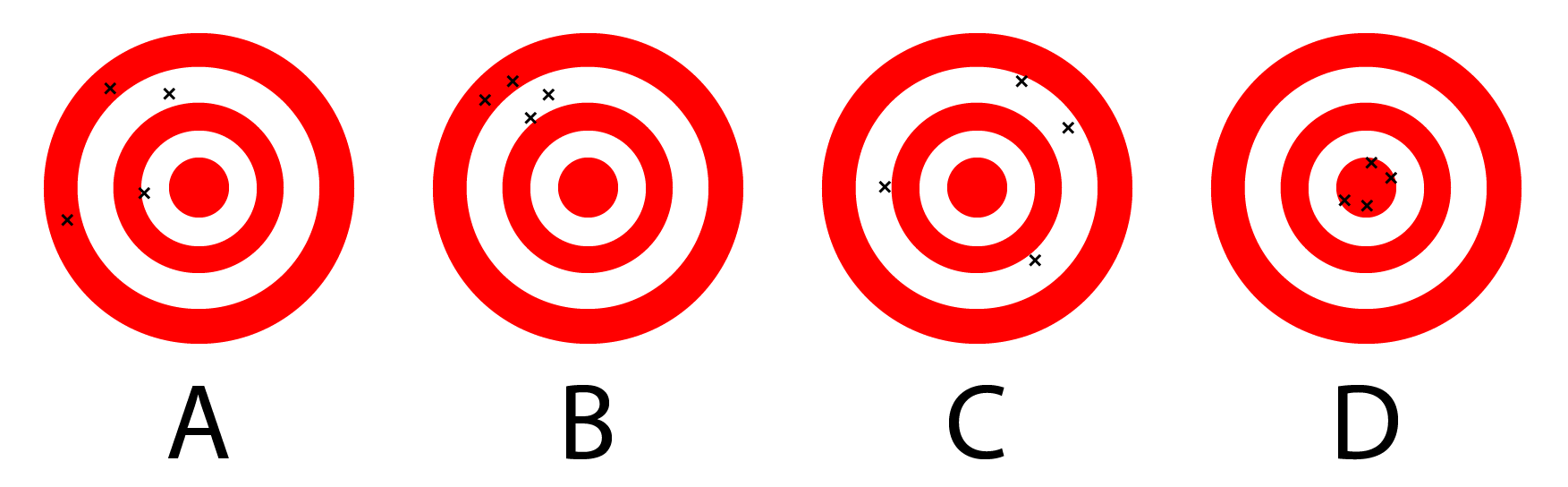
Let’s look at each player. Player A does not have a high accuracy and the darts are spread out. Player B does not throw near the bulls-eye but their throws are close together. Therefore, Player B would have low accuracy but better precision. Player C seems to have a higher accuracy than Players A and B, but their precision is poor. Finally, Player D has a high accuracy and high precision. Based on the picture, I would judge that Player D is the better player.
The goal is to choose an estimator with accuracy and precision. We discussed that being unbiased is analogous to accuracy. If we consider the precision of the estimator, a good measurement is the variance of the estimator.
Example 2.10 Consider the previous example where we have three potential estimators:
\[ \begin{align*} &\hat{p}_1 = \frac{X_1}{10}\\ &\hat{p}_2 = \frac{X_1 + X_2 + X_3}{30}\\ &\hat{p}_3 = \hat{p}_2 + 0.1 \end{align*} \]
where \(X_i \overset{iid}{\sim} \text{Bin}(10, p).\) Recall from our previous work that \(\hat{p}_1\) and \(\hat{p}_2\) are unbiased estimators of \(\theta\), and \(\hat{p}_3\) is a biased estimator. Find the variance of each estimator.
Solution
To find the variance of the estimators, we should recall three rules from STAT 414: - For a Binomial random variable \(X\), \(\text{Var}(X) = np(1-p).\) - \(\text{Var}(aX+b) = a^2 \text{Var}(X)\) for a random variable \(X.\) - If random variables \(X\) and \(Y\) are independent, then \(\text{Var}(X+Y) = \text{Var}(X) + \text{Var}(Y).\)
Now, let’s find the variance of \(\hat{p}_1\): \[ \begin{align*} \text{Var}(\hat{p}_1) &= \text{Var}\left(\frac{X_1}{10}\right)\\ &= \left(\frac{1}{10}\right)^2 \text{Var}(X_1)\\& = \frac{10p(1-p)}{100} \\&= \frac{p(1-p)}{10} \end{align*} \]
Next, find the variance of \(\hat{p}_2\): \[ \begin{align*} \text{Var}(\hat{p}_2) &= \text{Var}\left(\frac{X_1 + X_2 + X_3}{30}\right)\\& = \frac{1}{30^2} \text{Var}(X_1 + X_2 + X_3) \\ &= \frac{\text{Var}(X_1) + \text{Var}(X_2) + \text{Var}(X_3)}{30^2} \\&= \frac{10p(1-p) + 10p(1-p) + 10p(1-p)}{30^2} \\ &= \frac{30p(1-p)}{30^2}= \frac{p(1-p)}{30} \end{align*} \]
Finally, find the variance of \(\hat{p}_3\): \[ \begin{align*} \text{Var}(\hat{p}_3) &= \text{Var}(\hat{p}_2 + 0.1) = \text{Var}(\hat{p}_2) = \frac{p(1-p)}{30} \end{align*} \]
So, we found that both \(\hat{p}_1\) and \(\hat{p}_2\) are unbiased estimators. We found above that \(\text{Var}(\hat{p}_1)>\text{Var}(\hat{p}_2.\) Based on the two properties of estimators we learned so far, it seems like \(\hat{p}_2\) is the better estimator.
In the example above, we chose an unbiased estimator with the smallest variance. Would we ever use an estimator that is biased? And if so, why?
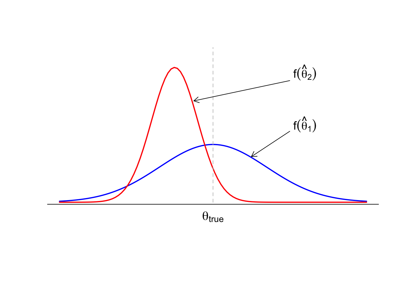
It can be the case that we can greatly reduce the variance by introducing a small amount of bias. For example, consider two estimators, \(\hat{\theta}_1\) and \(\hat{\theta}_2.\) Consider the graph of their pdfs.
We can see the pdf of \(\hat{\theta}_1\) is centered around the true value of \(\theta.\) However, \(\hat{\theta}_1\) has a larger variance. However, \(\hat{\theta}_2\) is not centered around the true value but has considerably lower variance.
Example 2.11 Consider the previous example where we have a random sample of size \(n\) from a Normal distribution with mean \(\mu\) and variance \(\sigma^2.\) We have shown that
\[\begin{align*} \hat{\sigma}^2_1=\frac{\sum_{i=1}^n (X_i-\bar{X})^2}{n} \end{align*}\]
is a biased estimator of \(\sigma^2.\) We also found that
\[\begin{align*} \hat{\sigma^2}_2=\frac{\sum_{i=1}^n(X_i-\bar{X})^2}{n-1} \end{align*}\]
is an unbiased estimator. We found that:
\[\begin{align*} E(\hat{\sigma^2}_1)=\frac{n-1}{n}\sigma^2 \end{align*}\]
However, as \(n\) approaches infinity, the expected value approaches \(\sigma^2.\) Therefore, \(\hat{\sigma}^2_1\) is asymptotically unbiased. Therefore, it may be the case that as the sample size gets larger, the bias of the estimator will go to 0.
Is there a measure that could help us to find a good balance between the bias of the estimator and also its variance? The answer is yes. One measure is the mean square error (MSE).
Def. 2.3 (Mean Square Error of a point estimator \(\hat{\theta}\)) The mean square error of a point estimator \(\hat{\theta}\) is defined as
\[\begin{align*} \text{MSE}(\hat{\theta})=E\left[(\hat{\theta}-\theta)^2\right] \end{align*}\]
The mean square error of an estimator is the average of the square of the distance between the estimator and the true parameter, \(\theta.\)
Based on the definition of MSE, it is obvious that a desirable estimator has the smallest mean square error.
The mean square error of \(\hat{\theta}\), is a function of both the bias and the variance of an estimator. It can be shown that
\[\begin{align*} \text{MSE}(\hat{\theta})=\text{Var}(\hat{\theta})-\left[\text{Bias}(\theta)\right]^2 \end{align*}\]
where \(\text{Bias}(\hat{\theta})\) is the bias of \(\hat{\theta}.\) You should convince yourself that the above relationship holds. It may be asked on an assignment.
Example 2.12 Consider our previous example with the following three estimators for the binomial parameter \(p\), with \(n=10.\) The estimators were: \[\begin{align*} & \hat{p}_1=\frac{X_1}{10}\\ & \hat{p}_2=\frac{X_1+X_2+X_3}{30}\\ & \hat{p}_3=\hat{p}_2+0.1 \end{align*}\] Find the MSE for each of the estimators.
Solution
Previously, we found the variance and expected value for each estimator. It is summarized here for convenience.
\[\begin{align*} & E(\hat{p}_1)=p, \qquad \text{Var}(\hat{p}_1)=\frac{p(1-p)}{10}\\ & E(\hat{p}_2)=p, \qquad \text{Var}(\hat{p}_2)=\frac{p(1-p)}{30}\\ & E(\hat{p}_3)=p+0.1, \qquad \text{Var}(\hat{p}_3)=\frac{p(1-p)}{30}\\ \end{align*} \]
To find the mean square errors, we need to find the bias of each estimator.
\[\begin{align*} & \text{Bias}(\hat{p}_1)=E(\hat{p}_1)-p=0\\ & \text{Bias}(\hat{p}_2)=E(\hat{p}_2)-p=0\\ & \text{Bias}(\hat{p}_3)=E(\hat{p}_3)-p=p+0.1-p=0.1\\ \end{align*}\]
Therefore, the MSEs are:
\[\begin{align*} & MSE(\hat{p}_1)=\text{Var}(\hat{p}_1)-\left[\text{Bias}(\hat{p}_1\right]^2=\frac{p(1-p)}{10}\\ & MSE(\hat{p}_2)=\text{Var}(\hat{p}_2)-\left[\text{Bias}(\hat{p}_2\right]^2=\frac{p(1-p)}{30}\\ & MSE(\hat{p}_3)=\text{Var}(\hat{p}_3)-\left[\text{Bias}(\hat{p}_3\right]^2=\frac{p(1-p)}{30}-0.1^2=\frac{p(1-p)}{30}-0.01\\ \end{align*}\]
Therefore, the estimator with the smallest MSE is \(\hat{p}_2.\)
In the next lesson, we will discuss another desirable property of an estimator, sufficiency.
2.3 Summary
This lesson introduced the idea of using sample data to estimate unknown population parameters. We focused on point estimation and explored what makes an estimator desirable by examining bias, variance, and mean squared error (MSE). Through examples and derivations, we learned how to evaluate and compare estimators using these properties. The lesson built a foundation for judging estimator quality in both theoretical and applied contexts.
Key Takeaways
- Bias measures how far an estimator’s average is from the true parameter.
- Variance captures the variability of an estimator across samples.
- Mean Squared Error (MSE) combines bias and variance to assess overall accuracy.
Comparing MSE helps decide which estimator is better in practice.