3+2

3-2

3*2

3/2

3^2

exp(3)

sqrt(3)

log(3)5 Maximum Likelihood Estimation (MLE) (Part II)
Point Estimation
Unbiased Estimation
Bias
Variance and Mean Square
Factorization
Sufficiency
Method of Moments
This lesson advances your understanding of maximum likelihood estimation (MLE) by focusing on its practical implementation, particularly through numerical methods in R. You will learn to compute MLEs for single and multiple parameter models using techniques such as grid search and the Newton-Raphson algorithm, with an emphasis on the optim function in R. Additionally, this lesson introduces essential R programming skills, including basic operations, vector and data frame manipulation, summary statistics, plotting, and working with statistical distributions like the normal and exponential. Through examples, you will explore how to evaluate likelihood and log-likelihood functions, simulate random variables, and estimate parameters numerically. By the end of this lesson, you will be proficient in applying MLE in real-world scenarios and leveraging R for statistical analysis, setting the stage for more advanced inference techniques.
Objectives
Upon completion of this lesson, you should be able to:
- Numerically estimate MLEs for a range of single parameter models and multiple parameter models using optim in R in situations where data values are given, and
- Use R to numerically simulate random variables from standard distributions, and also find pdfs, CDFs, and quantiles of standard distributions, including the normal, exponential, Poisson, geometric, and binomial distributions.
5.1 Introduction to R
5.1.1 Basic Operations in R
R can be used as a scientific calculator. The following shows a small subset of the calculator like functions that can be done in R.
Note that in R, and statistics and probability in general, the “log” function is, by default, the natural logarithm (base \(e\)). In mathematics, this is typically denoted by \(\ln(x)\), but in statistics, this is almost always denoted simply by \(\log(x)\).
One can see this from the following code:
e=exp(1)
e
[1] 2.718282## log base e of e = 1
log(e)[1] 1## log base e of 10 does NOT = 1
log(10)[1] 2.3025855.1.2 Defining and storing scalars and vectors
In general, you want to type your R code in a text file with the “.r” or “.R” extension, and then send lines or blocks of code to the R console. This lets you change code easily, save your work, and copy/paste it for use in other scenarios.
You will often want to store numbers as variables. You can then use those variables for calculations. Here’s a very simple example of multiplying two numbers together:
a=4

b=3

a*b
[1] 12We often want to work with multiple numbers, stored in a “vector” of numbers. R handles vectors (and matrices!) naturally. We can create a vector by using the c command in R (which stands for “concatenate”)
## Vectors

v=c(1,4,3,2)
v
[1] 1 4 3 2u=1:4
u[1] 1 2 3 4This has created two vectors, u and v, each with four elements. If we apply standard math operations to vectors, R’s default behavior is to apply those operations to each element. The code below illustrates this.
## element-wise operations
v+2
[1] 3 6 5 4v*2[1] 2 8 6 4u^2[1] 1 4 9 16u+v[1] 2 6 6 6u*v[1] 1 8 9 85.1.3 Subsetting vectors
We often have data or parameters stored in a vector, but only want to access one element, or a few elements, of that vector. Indexing in R is done using the square brackets: [ ]
## Subsetting vectors
v
[1] 1 4 3 2v[1][1] 1v[2][1] 4v[3][1] 3v[4][1] 2v[1:3][1] 1 4 3v[c(1,4)][1] 1 2v[c(3,4)][1] 3 25.1.4 Logical statements and the which command
One important way we will subset vectors is through logical arguments. R allows us to check whether a logical statement is TRUE or FALSE. This is most often done using the <, >, or == commands. Note that testing whether or not two numbers are equal must be done with double equal signs ==, not a single equal sign =, which is used to assign a value to a variable.
Here are some examples of checking logical statements in R. Note that logical statements can be applied elementwise to vectors, just like mathematical operations can.
## logical statements
3>4
[1] FALSE3>2[1] TRUE3==4[1] FALSE3==3[1] TRUEv[1] 1 4 3 2v>2[1] FALSE TRUE TRUE FALSEv==2[1] FALSE FALSE FALSE TRUEv>=2[1] FALSE TRUE TRUE TRUEA common task in statistical analyses (See Section 4 for examples!) is to find which elements of a vector satisfy certain criteria. The commands to do so in R revolve around the which command. Here are some examples:
## subsetting using logical arguments
v
[1] 1 4 3 2which(v>2)[1] 2 3v[which(v>2)][1] 4 3idx=which(v>2)
idx[1] 2 3v[idx][1] 4 35.1.5 Creating Data Frames
The R data.frame is a very important data structure. It allows you to store a “matrix” of data that is a mix of numeric columns (like response variables) and character columns (like human-readable names of treatments). Consider a farming example in which 10 plots were assigned either Fertilizer X (plots 1-5) or Fertilizer Y (plots 6-10). We will create a data frame that has this information in it, together with the response (corn yield at each plot).
First, we will create a numeric vector of the plot number. The code below shows you two equivalent ways to do this.
plot.ID=1:10

plot.ID=c(1,2,3,4,5,6,7,8,9,10)
Next, we will create the character vector of treatments. Note that you need to put letters in parentheses, or R will assume that the letter is a name of a vector or scalar already defined in R. See Section 3.2 for examples.
treatment=c("X","X","X","X","X","Y","Y","Y","Y","Y")

treatment=c(rep("X",5),rep("Y",5))
Now we will create a vector of responses
response=c(14,12,11,18,20,21,20,17,23,25)And finally, we will put these all together into a data.frame.
corn.yield=data.frame(plot.ID,treatment,response)

corn.yield
plot.ID treatment response
1 1 X 14
2 2 X 12
3 3 X 11
4 4 X 18
5 5 X 20
6 6 Y 21
7 7 Y 20
8 8 Y 17
9 9 Y 23
10 10 Y 255.1.6 Summary statistics in R
The summary function can tell you a lot about a data frame, as it computes the minimum, maximum, mean, and median of each numeric column.
summary(corn.yield) plot.ID treatment response
Min. : 1.00 Length:10 Min. :11.00
1st Qu.: 3.25 Class :character 1st Qu.:14.75
Median : 5.50 Mode :character Median :19.00
Mean : 5.50 Mean :18.10
3rd Qu.: 7.75 3rd Qu.:20.75
Max. :10.00 Max. :25.00 You can also use R to get means, variances, and standard deviations of whole vectors:
mean(response)[1] 18.1var(response)[1] 21.43333sd(response)[1] 4.629615or even subsets of vectors
mean(response[treatment=="X"])[1] 15mean(response[treatment=="Y"])[1] 21.2sd(response[treatment=="X"])[1] 3.872983sd(response[treatment=="Y"])[1] 3.033155.1.7 Simple Plotting in R
R can be used for plotting data as well. Having the data into a data.frame object can make plotting and data analysis easier. For example, we can plot a boxplot of the corn yield data using the boxplot command
boxplot(response~treatment,data=corn.yield,
        main="Boxplot of Corn Yield With Different Fertilizers",
        xlab="Fertilizer",ylab="Yield (kg)")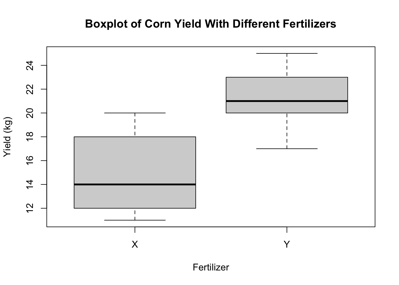
Histograms can be plotted using the hist command.
hist(response,main="Histogram of Corn Yield (All Plots)")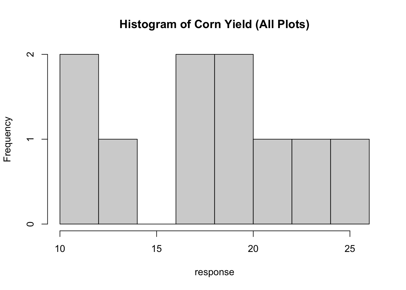
And numeric data can be plotted as a scatterplot using the plot command.
plot(x=plot.ID,y=response)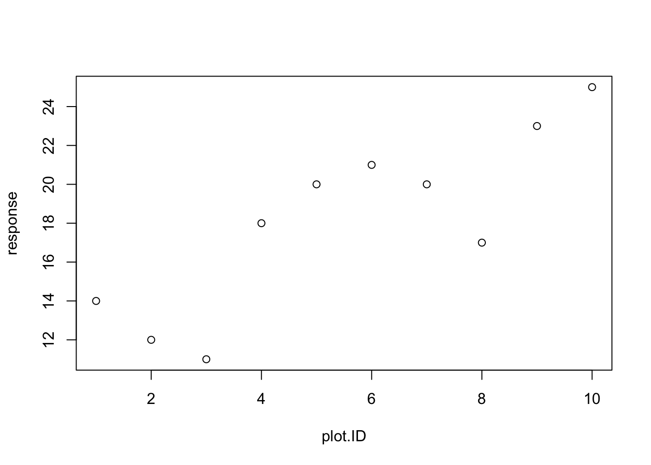
You will often need to include R graphics in your homework solutions. Once you have made the plot, you can right click on the figure in Rstudio, and then copy the image which can then be pasted into a Word document (or similar document).
5.1.8 Statistical Distributions in R
Help files in R
There are many functions in R - too many for any person to memorize all of the functions needed for most analyses. R also has a very robust system of documentation, as long as you know what to look for. In particular, if you know the name of a function that you need help with, R can help you very easily (see below). But if you don’t know what the name is for a function that does something you want to do, then your best bet is to search for that function on the internet using your favorite search engine.
For example, if you want to know how to find the CDF of a Normal distribution in R, searching something like “CDF normal distribution in R” will quickly give you many results that point you to the pnorm function.
Once you know the function you may want to use, you can access R’s help files for that function by typing help(pnorm) or ?pnorm into the R console. Note, that you should replace pnorm with whatever function you are looking for help with.
R Functions for Statistical Distributions
R is a great statistical software for working with distributions. Three main tasks related to random variables that R is very good at are:
Drawing random variables from a given distribution
Calculating the pdf or pmf or likelihood of a distribution at a given observed value
Calculating quantiles and cdfs of distributions.
In R, there is a pattern to functions related to a distribution. If a given distributions short name in R is “XXX”, then “rXXX” will draw a random variable from that distribution, “dXXX” will calculate the probability density function of that distribution, and “pXXX” will calculate the cumulative distribution function, and “qXXX” will calculate the quantile.
Examples from the Gaussian (Normal) Distribution
For example, let’s assume that each \(x_i \sim N(3,4)\) is an independent, normally-distributed random variable with mean 3 and variance 4. R’s normally-distributed variable “short name” is “norm”, so to draw one random variable we could use the following code:
rnorm(n=1,mean=3,sd=2)[1] 4.588832Note that R uses the standard deviation sd instead of the variance. If I wanted to draw 10 iid random variables, I could modify the n argument to rnorm:
rnorm(n=10,mean=3,sd=2) [1] 3.8443768 2.8336370 0.9059068 -1.2389454 5.3511716 4.8804865
[7] 4.8785879 3.4801860 1.0337144 4.7300503I can also assign these values to a variable for future use”
x=rnorm(n=1,mean=3,sd=2)

x
[1] 1.909684Now if I wanted to evaluate the pdf of a \(x \sim N(3,4)\) at a particular value \(u=2\), I can use the dnorm function:
dnorm(2,mean=3,sd=2)[1] 0.1760327The code above returns \(f_X(2)\). To get the CDF we use the pnorm function, with \(F_X(2) = P(X\le 2)\) being obtained by:
pnorm(2,mean=3,sd=2)[1] 0.3085375These functions all work on vectors as well. For example, if I wanted to evaluate the likelihood function of the ten simulated data points in “x”, I could do so by
dnorm(x,mean=3,sd=2)[1] 0.1719271The total likelihood of all the simulated random variables \(L(X_1,\ldots,X_{10}) = \prod_i f_X(X_i)\) would then be
prod(dnorm(x,mean=3,sd=2))[1] 0.1719271and the log-likelihood \(l(X_1,\ldots,X_10)=\sum_i log(f_X(X_i))\) could be calculated by
sum(log(dnorm(x,mean=3,sd=2)))[1] -1.760684R has an argument to dnorm to obtain the log-density instead of the density:
dnorm(x,mean=3,sd=2)[1] 0.1719271dnorm(x,mean=3,sd=2,log=TRUE)[1] -1.760684which is also often helpful.
Examples from the Exponential distribution
As a second example, consider the Exponential distribution \(z_i\sim Exp(\lambda)\). We can draw 30 random variables, each from \(z_i\sim Exp(2)\) (so \(E(z_i)=0.5\)) with the following
z=rexp(n=30,rate=2)
z
[1] 0.142767577 0.296127887 1.327931114 0.939315991 0.126033566 1.446248613
[7] 0.038309156 0.175018697 0.271329752 1.994453949 0.771627209 0.728734857
[13] 0.390166169 0.750427644 0.683243037 0.560096258 0.724887028 0.465139223
[19] 1.359739973 0.024589702 0.457575215 0.394187147 0.409137173 0.177320108
[25] 0.007190475 0.118036853 0.248750937 0.385974118 0.563551513 0.740833738Let’s get the mean and median of the simulated data
mean(z)[1] 0.5572915median(z)[1] 0.4333562which are similar to the theoretical mean (of \(1/\lambda=0.5\)) and median (of \(\ln(2)/\lambda=0.34657\))
Now let’s simulate 1000 random variables
z=rexp(n=1000,rate=2)This is too many to print, so let’s plot them with a histogram
hist(z)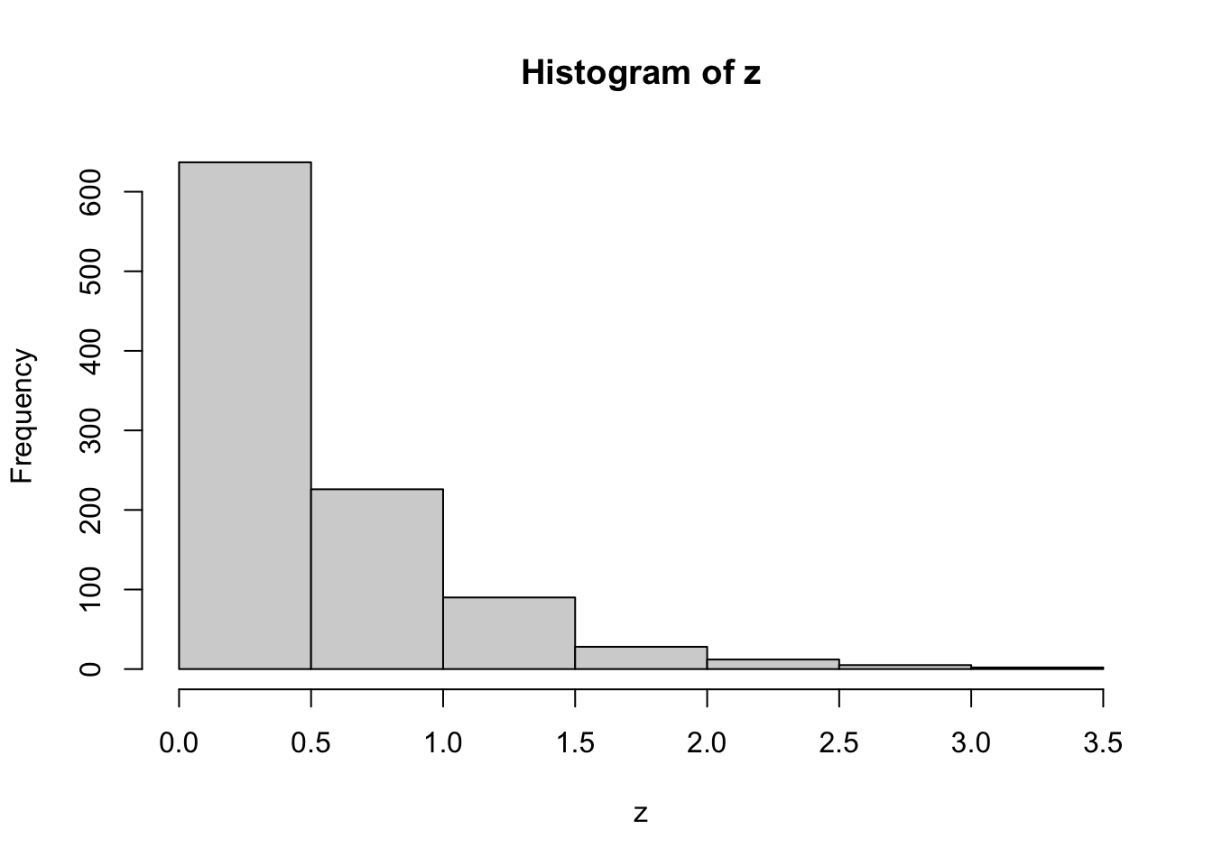
These look exponentially-distributed, as they should. We will now calculate multiple theoretical quantities of exponential random variables with rate 2, and compare them with estimates of these quantities from the simulated random variables \({z_i,i=1,2,...,1000}\).
First let’s look at values of the CDF - the cumulative distribution function. The probability of \(P(z<1)\) is \(F_Z(1)\), which in R is found using the pexp command
pexp(1,rate=2)[1] 0.8646647and the sample-based approximation to this is given by the number of sampled \(z_i\) that are less than or equal to 1, divided by the total number of samples (n=1000 here).
n.less.than.1=length(which(z<=1))
n.less.than.1
[1] 863cdf.val=n.less.than.1/1000
cdf.val[1] 0.863which is a close approximation to the true value shown above.
If we wanted the joint likelihood of \((z_1,z_2,...,z_1000)\), we could get it by \(f_Z(z_1,z_2,...,z_1000)=\prod_{i=1}^{1000} f_Z(z_i)=\prod_{i=1}^{1000} \lambda e^{-\lambda z_i}\), which we can obtain directly in R
prod(2*exp(-2*z))[1] 4.918477e-138or can be obtained using the dexp command
prod(dexp(z,rate=2))[1] 4.918477e-1385.2 Numeric Maximum Likelihood Estimation
Now back to MLEs!
In the previous section, we showed an example where the maximum likelihood estimator could not be solved analytically and we require numerical optimization to solve the equation. In this section, we present two methods to find the maximum likelihood estimate numerically. The first method is to find it, using R, by a grid search. The other uses the optim function in R.
5.2.1 MLE Through Grid Search
One way to find the MLE is through a grid search. The idea is to use software, such as R, to make the calculations for you. We know the underlying distribution and thus can find the likelihood function. Then, given a set of data and possible values of the unknown parameter, \(\theta\), we can find the value of \(\theta\) that maximizes the likelihood.
To illustrate this, let’s assume that we have the following data points. Suppose the data come from an exponential distribution with unknown mean \(\theta\).
x=c(1,  5, 10,  1,  3, 11, 10, 23,  2,  6,  1, 24,  6, 11, 19)
x
> [1] 1 5 10 1 3 11 10 23 2 6 1 24 6 11 19hist(x,breaks=7)
If we don’t know the parameter \(\theta\), we could try to estimate it with maximum likelihood estimation, where the estimate is the value that maximizes the likelihood function \[\hat{\theta}=\text{argmax}{L(\theta,\mathbf{x})}\] We could try just picking a few values of \(\theta\) to try:
lik.exp.2=function(theta,x){
  prod(dexp(x,rate=1/theta))
}
lik.exp.2(2,x)
[1] 4.017603e-34lik.exp.2(10,x)[1] 1.674493e-21lik.exp.2(20,x)[1] 3.949042e-23Out of this small collection of values, \(\theta=10\) gives the highest likelihood.
To try a sequence of values, we’ll build a “for” loop. Our goal is to end up with a vector of likelihood values for a sequence of \(\theta\) values. We start by specifying the \(\theta\) values we want to consider.
theta.vals=seq(1,100,by=0.1)
theta.vals
[1] 1.0 1.1 1.2 1.3 1.4 1.5 1.6 1.7 1.8 1.9 2.0 2.1 2.2 2.3 2.4 2.5 2.6 2.7 2.8
[20] 2.9 3.0 3.1 3.2 3.3 3.4
...
[1] 97.6 97.7 97.8 97.9 98.0 98.1 98.2 98.3 98.4 98.5 98.6 98.7
[13] 98.8 98.9 99.0 99.1 99.2 99.3 99.4 99.5 99.6 99.7 99.8 99.9
[25] 100.0We then create an empty vector of likelihood values (we’ll fill in the values later)
lik.vals=rep(NA,length(theta.vals))We can now make a for loop that (1) evaluates the likelihood function for each value of theta, and (2) saves that value in the correct spot in lik.vals.
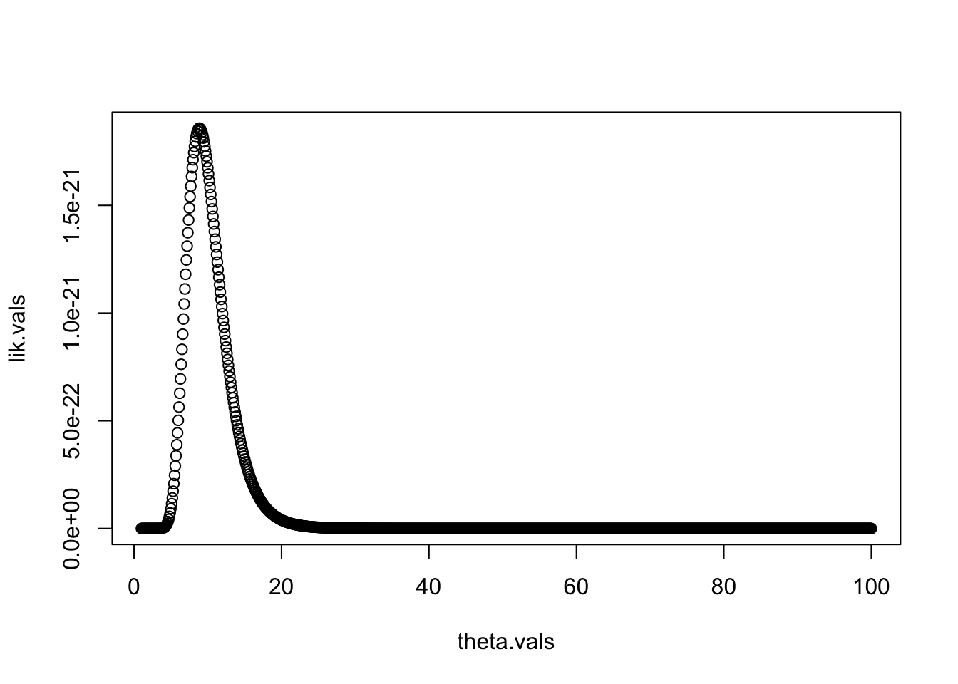
This approach is often called a “grid search”, as we are searching over a wide range of values of our parameters. From the plot, we can see that the MLE is somewhere near 10. We can find the best value of \(\theta\) out of those we tried by using the which.max command, which finds the index of the maximum value in a vector.
idx.mle=which.max(lik.vals)
idx.mle
[1] 80theta.hat.grid=theta.vals[idx.mle]
theta.hat.grid[1] 8.9Thus, given the values that we tried, our MLE is \(\hat{\theta}_{grid}=8.9\).
This is a crude method of finding the MLE. The next method we present is more comprehensive.
5.2.2 Numerical MLE: The Idea
A better alternative to the grid search above is to use one of many iterative methods for maximizing a function. One such method is called the Newton-Raphson algorithm, also sometimes called Newton’s Method.
Numerical optimization is a huge field! There are many optimization algorithms to choose from. Most of the optimization algorithms share some characteristic steps. They involve:
Requiring a starting value for the parameters, \({\theta}=(\theta_1, \theta_2, \ldots, \theta_p)\), denoted \({\theta}_0\).
Interactively finding a sequence of new parameters, \({\theta}^{(1)}, {\theta}^{(2)}, \ldots\)
Stops when \({\theta}^{(k)}\) is “close” to a local maximum.
The algorithm we will consider in this class is the Newton-Raphson Algorithm or Newton’s Method.
5.2.3 Newton’s Method Approach Idea
The idea is maximizing the log likelihood function, \(\ell(\theta)\). We do this by finding \(\frac{d}{d\theta} \ell(\theta)=0\). The derivative, \(\frac{d}{d\theta} \ell(\theta)=0\) is just a function of \(\theta\), so let’s define it as \(h(\theta)=\frac{d}{d\theta} \ell(\theta)=0\).
We need to find the “root” of \(h(\theta)\). In other words, we need to find a \(\theta\) such that \(h(\theta)=0\).
We get closer to the root (\(h(\theta)=0\)) by approximating \(h(\theta)\) with a tangent like at the current value of \(\theta\). So we start with a value, \(\theta^{(0)}\). We evaluate \(h(\theta^{(0)}=\frac{d}{d\theta}\ell(\theta^{(0)})\). The tangent line at \(\theta^{(0)}\) is
\[\begin{align*} y=h^\prime(\theta^{(0)})(\theta-\theta^{(0)})+h(\theta^{(0)}) \end{align*}\]
Setting \(y=0\) gives us where this tangent line hits 0. \[\begin{align*} 0=h^\prime(\theta^{(0)})(\theta-\theta^{(0)})+h(\theta^{(0)}) \end{align*}\]
Now, we solve for \(\theta\) to get: \[\begin{align*} \theta^{(1)}=\theta^{(0)}-\frac{h(\theta^{(0)})}{h^\prime(\theta^{(0)})} \end{align*}\]
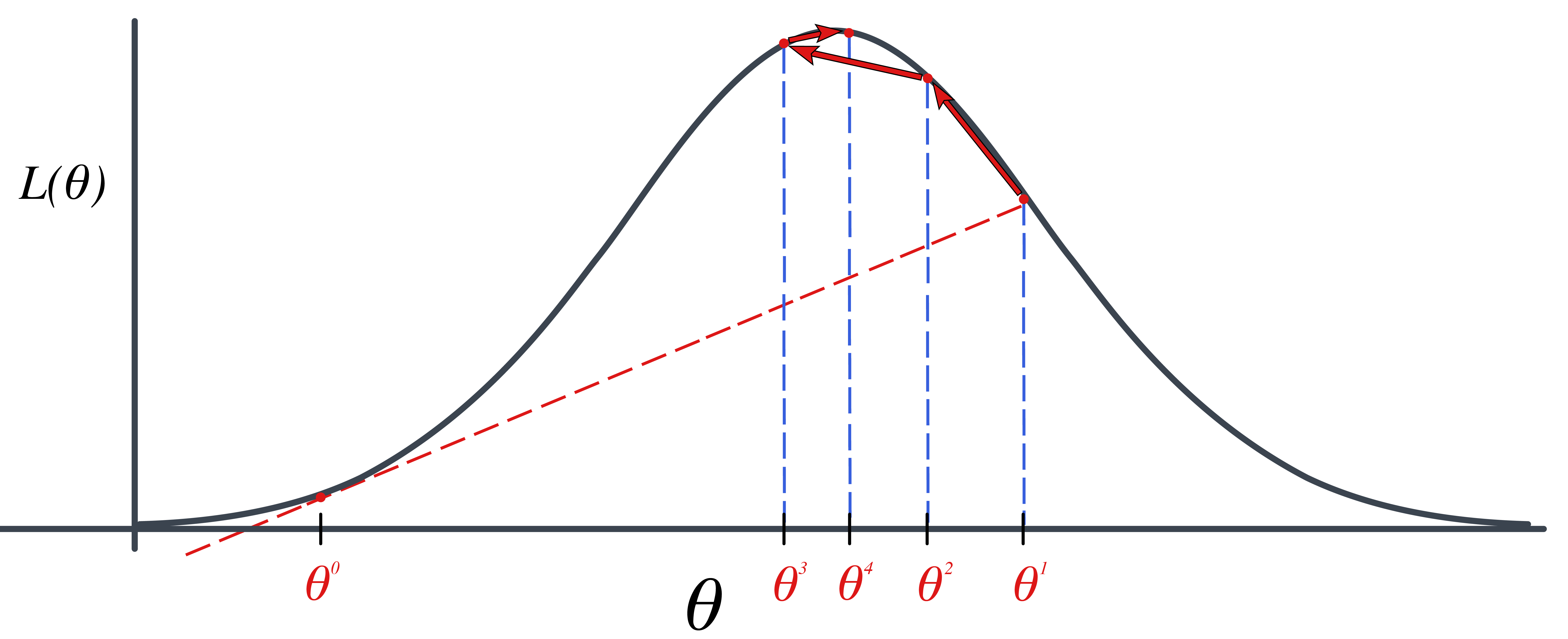
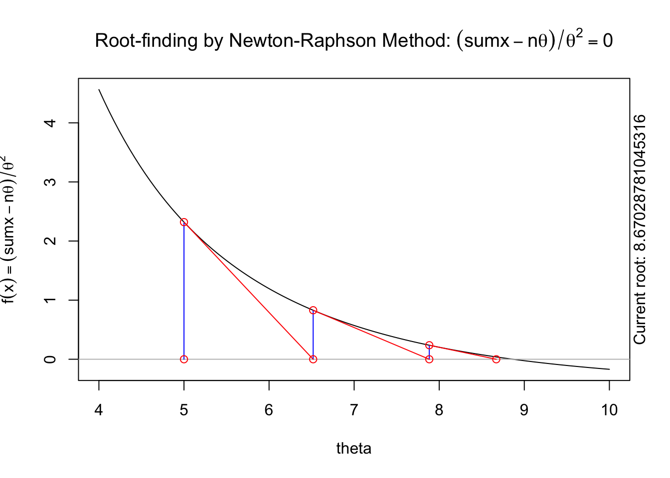
The following animation displays how this works to find the root. We start with an initial value of \(\theta\), \(\theta^{(0)}\) (blue dot). We evaluate the log likelihood function at that value. Then we find the tangent line for the initial value. Find where the tangent line crosses the x-axis. That point becomes our “new” value of \(\theta\), \(\theta^{(1)}\). Then, we repeat the same steps we did for the initial \(\theta\) value. We keep going until we find the maximum.
The steps are:
Specify a starting value, \(\theta^{(0)}\).
For \(t=1, 2, \ldots\) find: \[\begin{aligned} \theta^{(t+1)}=\theta^{(t)}-\frac{h(\theta^{(t)})}{h^\prime(\theta^{(t)})}=\theta^{(t)}-\frac{\frac{d}{d\theta}\ell(\theta^{(t)})}{\frac{d^2}{d\theta^2}\ell(\theta^{(t)})}\end{aligned}\]
5.2.4 Numerical Optimization in R
This section is meant to give you some intuition for how numerical optimization works using the R function, optim. In general, we will just USE existing algorithms, so most of your homework will not focus on understanding how algorithms like Newton’s method work. The next subsection (Numerical Optimization) contains the most useful code to use algorithms like Newton’s method to find MLEs. This subsection is meant to help you understand what is happening under the hood of optim and other numerical optimization routines.
If our goal is to maximize the likelihood function \(L(\theta,\mathbf{x})\), we could similarly maximize the log-likelihood function
This maximum could be found by first identifying any critical points that satisfy \(\frac{d}{d\theta}\ell(\theta)=\ell'(\theta)=0\) Thus, we need to find the values of \(\theta\) which are the roots of \(\ell'(\theta)\) - the values of \(\theta\) that make the function \(\ell'(\theta)\) equal zero.
Newton’s method is a root finding algorithm that works by iteratively approximating the function by a line. The details of Newton’s method are covered in the lectures, with the algorithm being as follows. Given a starting value \(\theta^{(0)}\), we iteratively update \(\theta^{(t)}\) as follows \[ \theta^{(t+1)}=\theta^{(t)} - \frac{\ell'(\theta^{(t)})}{\ell''(\theta^{(t)})}\] Let’s write functions to evaluate the first and second derivatives of the log-likelihood function. Note that R can’t directly calculate derivatives of a function, so we do the algebra and then code these into R functions \[ \ell'(\theta)=\sum_{i=1}^n\left(\frac{-\theta+x_i}{\theta^2} \right)=\sum_{i=1}^n (x_i-\theta)\theta^{-2}\] \[ \ell''(\theta)=\sum_{i=1}^n\left(\frac{-2x_i+\theta}{\theta^3} \right) \]
R functions to evaluate these are
l.first.der=function(theta,x){
  sum((x-theta)*theta^(-2))
}
l.scnd.der=function(theta,x){
  sum((-2*x+theta)/theta^3)
}
sumx=sum(x)
n=length(x)
And Newton’s method can be done by iterating:
## starting value
theta0=5
## first iteration
theta1=theta0-l.first.der(theta0,x)/l.scnd.der(theta0,x)
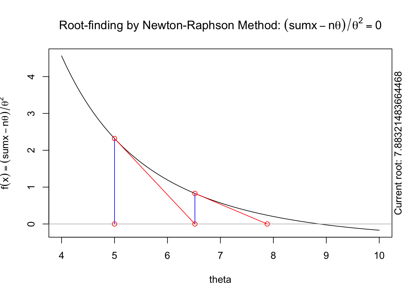
theta1[1] 6.518325## 2nd iteration
theta2=theta1-l.first.der(theta1,x)/l.scnd.der(theta1,x)
theta2[1] 7.883215## 3rd iteration
theta3=theta2-l.first.der(theta2,x)/l.scnd.der(theta2,x)
theta3[1] 8.670288## 4th iteration
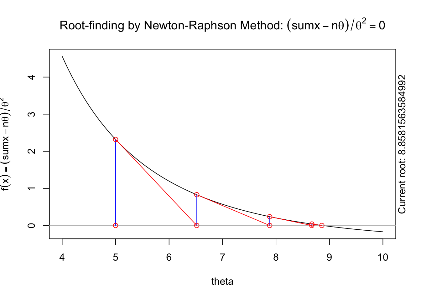
theta4=theta3-l.first.der(theta3,x)/l.scnd.der(theta3,x)
theta4[1] 8.858156## 5th iteration
theta5=theta4-l.first.der(theta4,x)/l.scnd.der(theta4,x)
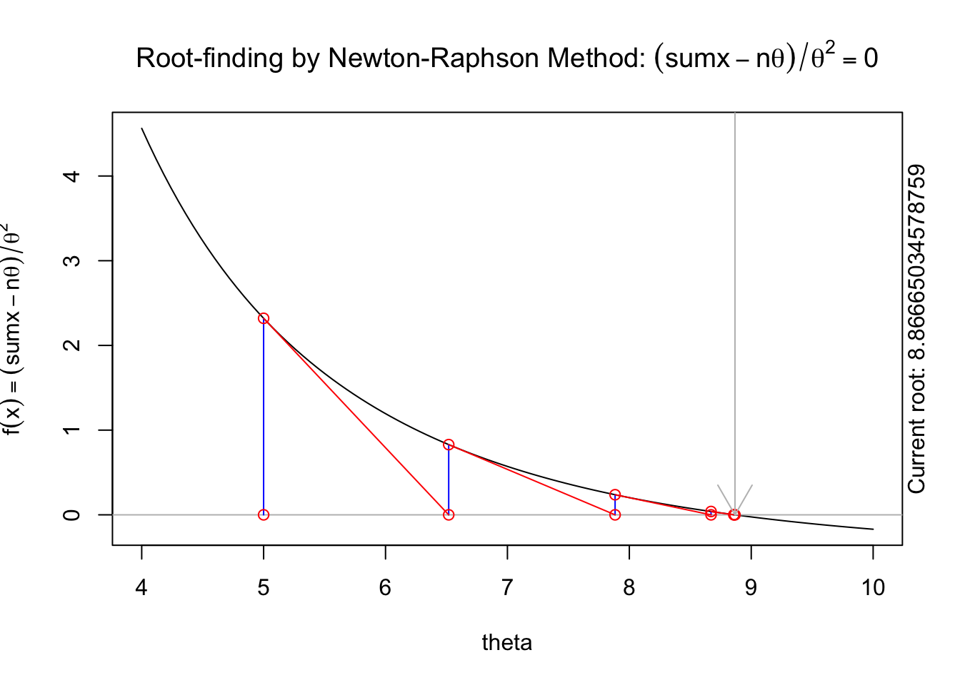
theta5[1] 8.86665## 6th iteration
theta6=theta5-l.first.der(theta5,x)/l.scnd.der(theta5,x)
theta6[1] 8.866667## 7th iteration
theta7=theta6-l.first.der(theta6,x)/l.scnd.der(theta6,x)
theta7[1] 8.866667## 8th iteration
theta8=theta7-l.first.der(theta7,x)/l.scnd.der(theta7,x)
theta8[1] 8.866667You can see that successive iterations seem to be converging on a value near 8.866667, which is similar to what we found in our grid search.
A visual illustration of Newton’s method is found in the animation R package. The following code won’t display online, but if you run it in your R console it will produce a nice illustration of Newton’s method.
install.packages("animation")
library(animation)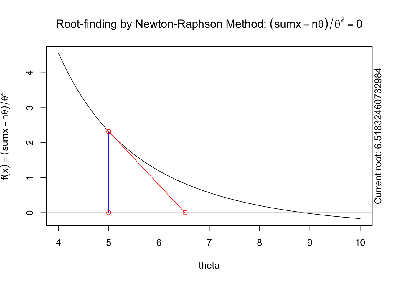
5.2.5 Numerical MLE in R
The previous section described and implemented two approaches to numerically approximating the maximum likelihood estimate. In this section, we will describe a more robust, general purpose approach to optimization using optim in R.
optim in R performs general numeric optimization. We will begin by considering a simple, contained use case for optim: using optim for maximum likelihood estimation. Consider the general case where \[x_i\sim f_X(x_i;\boldsymbol\theta)\] where \(\boldsymbol\theta=(\theta_1,\theta_2,...\theta_p)\) is a vector of all parameters in the model. Our goal is to find the MLEs of \(\boldsymbol\theta\). In this situation, optim takes as inputs the following
A set of initial values for \(\boldsymbol\theta\). This is a vector of initial guesses for each parameter in the model. In most cases, you do NOT need to think hard about the initial values, but you DO need to make sure that your initial values are valid. For example, if \(x_i\sim N(\mu,\sigma^2)\), then your initial value for \(\sigma\) must be a positive number, which your initial value for \(\mu\) could be any number.
A function to evaluate the negative log-likelihood of the data for a set of parameters. Note that we are working with the NEGATIVE log-likelihood instead of the standard log-likelihood - this is because
optimis coded to minimize by default, so the MLE of \(\boldsymbol\theta\) will maximize the log-likelihood but minimize the negative log-likelihood.
Important!
This function MUST have as its first input a VECTOR of ALL PARAMETERS. Any other inputs can be in any format.
We will first look at two examples that fit this framework, and then we’ll put together a code template that can be used for other problems.
Example 5.1 To illustrate finding numerical MLEs, we first consider data from an exponential distribution. We assume that the following 15 data points come from an exponential distribution with an unknown rate parameter \(\theta\), so \(x_i\sim Exp(\theta)\), with data
x=c(1,  5, 10,  1,  3, 11, 10, 23,  2,  6,  1, 24,  6, 11, 19)
x
[1] 1 5 10 1 3 11 10 23 2 6 1 24 6 11 19hist(x,breaks=7)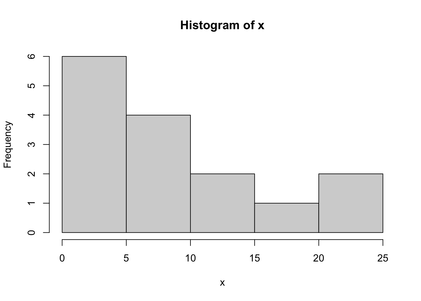
We first write an R function to evaluate the negative log-likelihood of the data. We’ll use dexp from R to evaluate the log-likelihood, with the log=TRUE option
nll.exp=function(theta,x){
  -sum(dexp(x,rate=1/theta,log=TRUE))
}
We break down this function piece by piece. The code: dexp(x,rate=1/theta) would evaluate the likelihood (PDF) of each data point in x given a value for theta, and so the code dexp(x,rate=1/theta,log=TRUE) evaluates the log-likelihood of each data point. Summing these up is done using the sum(...) command, and putting a negative sign in front returns the negative log-likelihood of the data.
We can then use optim to find the MLE of \(\theta\). We’ll first show the code, and then break down each piece.
out=optim(2,nll.exp,x=x)The syntax of optim is as follows. The first input needs to be a starting value for all parameters. As we only have one parameter, \(\theta\), we supply one starting value. This could be any number that is valid for the exponential distribution. Since the parameter \(\theta\) must be positive, we supply a positive initial value of \(\theta^{(0)}=2\) in the code above.
The second input is the NAME of the negative loglikelihood function we just wrote. As we called this nll.exp, this is what goes into optim in the second input slot. The third (and others if needed) inputs to optim are any extra inputs needed for the negative loglikelihood function. Our nll.exp function requires two inputs: theta and x. The first input, theta, is essentially supplied by our starting value. The second input, x, is a vector of the data. To tell optim what values to use for x, we put as a third input into optim the argument x=x. The left hand side x is the name of the input in the nll.exp function. The right hand side is the name of the data values (we called these x as well). In our following example, we’ll try to make this more clear.
The output of optim has multiple warnings. In general, you can IGNORE MOST WARNINGS FROM OPTIM! The warnings we have here are because optim, as part of its optimization algorithm, tried some values of \(\theta\) that were negative. These produced NA values when trying to evaluate the loglikelihood, but optim is coded in a way to try different values when this happens. We could avoid these warnings by specifying some options in optim, but for most simple cases, the result will NOT be different, and so we can almost always IGNORE WARNINGS FROM OPTIM.
optims output is as follows
out$par
[1] 8.865625
$value
[1] 47.73448
$counts
function gradient
30 NA
$convergence
[1] 0
$message
NULLThere are a few relevant pieces of this output.
out\$paris the MLE - the value of the parameter(s) that maximize the likelihood (and thus minimize the negative loglikelihood)out\$valueis the actual negative loglikelihood when evaluated at the MLE. So if we rannll.exp(0.112793,x)we would get 47.73448. In most applications, this can be ignored.out\$countsis the number of iterations of the optimization algorithm run. Here we see that the algorithm ran for 32 iterations before meeting a stopping criteria. This can almost always be ignored.out\$convergenceis given a value of0if the algorithm converges to its internal criteria. This is the result you want. Ifconvergencehas a value of1, then the algorithm has NOT converged, and we should NOT trust the value of the MLE.out\$messagecan most often be ignored.
Note that if we try different starting values, we may have slightly different results. For example, choosing a starting value of \(\theta^{(0)}=0.5\) gives
out2=optim(0.5,nll.exp,x=x)
out2
$par
[1] 8.86875
$value
[1] 47.73448
$counts
function gradient
34 NA
$convergence
[1] 0
$message
NULLwhich gives a very slightly different MLE (8.6875 vs 8.65625). If the difference is not trivial, one should take the value that gives the SMALLER negative log-likelihood value (shown in out$value).
In general, when looking at optim output, one should do the following:
- Check to see that
convergenceequals 0. - Then read off the MLEs from
par
Example 5.2 (MLE Example: The Normal Distribution) We’ll now give a different example using the Normal distribution. This time we will simulate some data from known parameters
mu.true=-3
s2.true=16

set.seed(123)
y=rnorm(30,mean=mu.true,sd=sqrt(s2.true))

hist(y)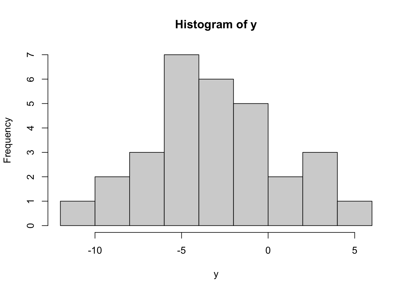
y [1] -5.2419026 -3.9207100 3.2348333 -2.7179664 -2.4828491 3.8602599
[7] -1.1563352 -8.0602449 -5.7474114 -4.7826479 1.8963272 -1.5607447
[13] -1.3969142 -2.5572691 -5.2233645 4.1476525 -1.0085981 -10.8664686
[19] -0.1945764 -4.8911656 -7.2712948 -3.8718997 -7.1040178 -5.9155649
[25] -5.5001571 -9.7467732 0.3511482 -2.3865075 -7.5525477 2.0152597This results in 30 values, each satisfying \(y_i\sim N(-3,16)\). We will now pretend that we do NOT know the true mean and variance, and numerically estimate these. We first write a negative log-likelihood function, with the first input being a vector of all parameters
nll.norm <- function(theta,y){
    ## get parameters
    mu=theta[1]
    s2=theta[2]
    ## calculate loglikelihood
    loglik=sum(dnorm(y,mean=mu,sd=sqrt(s2),log=TRUE))
    ## return negative loglikelihood
    -loglik
}
Note that our first input, called theta, is a vector with the first element the mean \(\mu\), and the second element the variance \(\sigma^2\). These are the parameters we need to estimate. In our exponential example above, we only had a single parameter, but here where we have two parameters, we need to first “unpack” the parameters from theta.
Note also that we wanted to find the MLE of \(\mu\) and \(\sigma^2\), but R’s dnorm function takes as an input the mean (\(\mu\)) and the STANDARD DEVIATION (\(\sigma\)), not the variance \(\sigma^2\). So in the dnorm statement, we specified the standard deviation sd as sd=sqrt(s2), the square root of the variance.
We now use optim to find the MLEs. We need a vector of starting values. For \(\mu\) we can use anything, while for \(\sigma^2\) we should have a positive number, so we’ll choose a starting value of \(\theta=(-1,1)\).
out=optim(c(-1,1),nll.norm,y=y)
out
$par
[1] -3.186135 14.885294
$value
[1] 83.07392
$counts
function gradient
77 NA
$convergence
[1] 0
$message
NULLSince the convergence is 0, we know that optim has passed its internal convergence checks, and we can trust the results. The MLEs are in par, and the order of the two MLEs is the same as the order of \(\theta\) - our vector of parameters. Since \(\mu\) was first, the MLE for \(\mu\) is the first number, and \(\hat{\theta}_{ML}=-3.186\). Similarly, the MLE for \(\sigma^2\) is \(\hat{\sigma^2}_{ML}=14.885\).
5.3 Summary
This lesson deepened your understanding of maximum likelihood estimation (MLE) by focusing on its numerical application and implementation in R. We explored how to construct and maximize likelihood and log-likelihood functions for single and multiple parameter models, using both analytical and numerical approaches.
Key techniques included the grid search method and the Newton-Raphson algorithm, with practical implementation through R’s optim function for finding MLEs. The lesson also introduced essential R programming skills, such as performing basic operations, manipulating vectors and data frames, generating summary statistics, creating visualizations like histograms and boxplots, and working with statistical distributions (e.g., normal and exponential) to simulate data and compute probabilities.
Through examples, you learned to handle real-world data scenarios, such as estimating parameters for exponential and normal distributions. These skills provide a robust foundation for applying MLE in statistical inference and prepare you for advanced topics like confidence intervals and hypothesis testing.