10  Hypothesis Tests (Part II)

This lesson picks up where our first look at hypothesis testing left off. We move beyond single‑sample tests to compare two populations, explore lesser‑known examples, and show how confidence intervals and hypothesis tests are two sides of the same coin. You’ll also learn why test quality hinges on power—the probability of catching a real effect—and how factors like sample size, significance level (\(\alpha\)), and effect size work together. Finally, we preview the Wald test, a general method that leverages maximum‑likelihood estimators when classic test statistics are hard to derive.

Objectives

Upon completion of this lesson, you should be able to:

1. Link confidence intervals to hypothesis tests,
2. Determine the Power of a test,
3. Find the sample size required for a given significance level and desired power,
4. Numerically construct simple hypothesis tests focused on parameters estimated using numerical maximum likelihood inference in R

10.1 Other Hypothesis Test Examples

In this section, we will continue with some examples of hypothesis tests that may not be as familiar as the ones we have seen so far.

Example 10.1 Part I
Suppose we have a random sample of size \(n=8\) from a Uniform distribution over the interval \((0, \theta)\). We wish to test the following hypotheses: \[\begin{align*} H_0:\theta=2 \text{ versus }H_a:\theta<2 \end{align*}\] Derive a statistical test for these hypotheses.

Solution

We have step 1 already defined for us. The next step is to set a significance level. Let’s set the probability of a Type I error to be \(\alpha=0.10\).

The next step is to find the test statistic. We need to know the distribution of the test statistic. A logical choice for the statistic would be the maximum order statistic. If the null hypothesis is true, the largest order statistic, \(Y_n=Y_8\), will be “close” to \(\theta=2\), and values of \(Y_8\) that are much smaller than \(\theta=2\) would be evidence in favor of the alternative hypothesis, \(H_a:\theta<2\).

The decision rule would be something like reject \(H_0:\theta=2\) if \(Y_8\le c\) where \[\begin{align*} \alpha=0.1=P(Y_8\le c|H_0\text{ is true}) \end{align*}\]

We know that the order statistic has the following distribution:

\[\begin{align*} f_{y_n}(y)=\frac{n}{\theta^n}y^{n-1}=\frac{8}{\theta^8}y^7, \qquad 0\le y\le \theta \end{align*}\]

Under the null hypothesis, the distribution is: \[\begin{align*} f_{y_8}(y)=\frac{n}{2^n}y^{n-1}=\frac{8}{2^8}y^7=\frac{1}{32}y^7, \qquad 0\le y\le 2 \end{align*}\]

Going back to our decision rule, we reject if \(P(Y_8\le c|H_0)=0.1\). Putting this all together, we can find \(c\).

\[\begin{align*} 0.1=\int_0^c \frac{1}{32}y^7dy=\frac{1}{256}c^8 \end{align*}\]

Solving for \(c\), we get: \[\begin{align*} c=\sqrt[8]{25.6}\approx 1.4998 \end{align*}\]

Thus, we reject the null hypothesis, at the \(\alpha=0.1\) level, if \(Y_8\le 1.4998\).

Part II

We have the following observations from a Uniform distribution over the interval \((0, \theta)\).

\[0.3977\ 0.9518\ 0.4598\ 0.3963\ 0.5222\ 0.8519\ 0.5270\ 0.2767\]

Test the hypotheses \(H_0: \theta=2\) vs. \(H_a: \theta<2\).

Solution

The maximum order statistic is 0.8519. Since it is less than 1.4998, we reject the null hypothesis. We conclude, that at the \(\alpha=0.1\) level, there is sufficient evidence the population parameter \(\theta\) is less than 2.

Example 10.2 Four measurements, 2, 0, 1, 0, are taken on a Poisson random variable \(X\) for the purpose of testing \[\begin{align*} H_0:\lambda=0.8 \text{ versus } H_a: \lambda>0.8 \end{align*}\]

Derive a statistical test for these hypotheses at the significance level of 10%.

Solution

The first two steps for hypothesis testing are given in the problem. Therefore, the next step is to calculate the test statistic. We have seen before that \(\bar{X}\) is a sufficient statistic for \(\lambda\). We have also found in 414 that \(\sum_{i=1}^4 X_i\) is a Poisson random variable with parameter \(\sum_{i=1}^4 \lambda=4\lambda\). For this example, let’s consider the sum as the test statistic.

If the distribution of the sum is Poisson \(4\lambda\), then we can translate our original hypotheses to:

\[\begin{align*} H_0: 4\lambda=4(0.8)=3.2 \text{ versus }H_a: 4\lambda>3.2 \end{align*}\]

Setting up the decision rule, we want to reject the null hypothesis if \(\sum x_i>c\), where \[\begin{align*} P\left(\sum X_i>c | H_0 \text{ true }\right)=0.1 \end{align*}\]

Recall that the Poisson distribution. Therefore, we may not get the exact \(\alpha\) level we desire. The table below shows the pmf of a Poisson random variable with \(\lambda=3.2\). The third column is the \(P(\sum X_i>x)\) for the value \(x\).

\(x\)	\(P(X=x)\)	\(P(X>x)=1-P(X\le x)\)
0	0.0408	0.9592
1	0.1304	0.8288
2	0.2087	0.6201
3	0.2226	0.3975
4	0.1781	0.2194
5	0.1140	0.1054
6	0.0608	0.0446
7	0.0278	0.0168
8	0.0111	0.0057
9	0.0040	0.0018
10	0.0013	0.0005
11	0.0004	0.0001
12	0.0001	0.0000
13	0.0000	0.0000

We want to get as close to \(\alpha=0.1\) as possible. The value that is closest is \(P(\sum X_i>5)=0.1054\). Therefore, at a significance level of \(\alpha=0.1055\), the decision rule to reject the null hypothesis is when \(\sum x_i\ge 6\).

Using the given data, the sum is \(Y=2+0+1+0=3\). Since the sum is not greater than or equal to 6, we fail to reject the null hypothesis. At the \(\alpha=0.1055\) level, there is insufficient evidence to conclude that \(4\lambda>3.2\) or equivalently, \(\lambda>0.8\).

10.2 Linking Confidence Intervals to Hypothesis Tests

At this point, we have demonstrated how to find interval estimates for unknown parameters and how to test for specific values of the unknown parameters. Is there any connection between the interval estimates and hypothesis tests? The answer is yes!

So far in this class, we have discussed only two-sided confidence intervals, i.e. intervals with an upper bound and a lower bound. We will focus our discussion on these intervals and two-sided tests. However, we can apply what we learn here to right-tailed or left-tailed confidence intervals and one-sided hypothesis tests.

As usual, lets consider an example.

Example 10.3 Let’s revisit a previous example. It is assumed that the mean systolic blood pressure is \(\mu = 120\) mm Hg. In the Honolulu Heart Study, a sample of \(n=100\) people had an average systolic blood pressure of 130.1 mm Hg with a standard deviation of 21.21 mm Hg. Find a 95% confidence interval for the population mean systolic blood pressure.

Solution

The 95% confidence interval is: \[\begin{align*} \bar{x}\pm t_{0.025, 99}\frac{s}{\sqrt{n}} \end{align*}\]

With the given information, we know, the interval is: \[\begin{align*} 130.1\pm 1.984\left(\frac{21.21}{\sqrt{100}}\right)=130.1\pm 4.2081=(125.8919, 134.3081) \end{align*}\]

We are 95% confident that the population mean systolic blood pressure is between \((125.8919, 134.3081)\).

Previously, we asked: Is the group significantly different (with respect to systolic blood pressure!) from the regular population? We tested the hypotheses: \[\begin{align*} H_0: \mu=120 \text{ versus }H_a: \mu\ne 120 \end{align*}\]

The test statistic was \(t=4.76\). The p-value for this test \(P(T>4.76)+P(T<-4.76)\approx 0.000\).Therefore, we rejected the null hypothesis at the \(\alpha=0.05\) level.

If we look at the confidence interval, we see that the value of 120 is NOT in the confidence interval. Is this a coincidence?

The critical region approach for the \(\alpha=0.05\) hypothesis test tells us to reject the null hypothesis that \(\mu=120\):

\[\begin{align*} \text{ if }t=\dfrac{\bar{x}-\mu_0}{s/\sqrt{n}}\geq 1.9842 \text{ or if }t=\dfrac{\bar{x}-\mu_0}{s/\sqrt{n}}\leq -1.9842 \end{align*}\]

which is equivalent to rejecting: \[\begin{align*} \text{ if }\bar{x}-\mu_0 \geq 1.9842\left(\dfrac{s}{\sqrt{n}}\right) \text{ or if }\bar{x}-\mu_0 \leq -1.9842\left(\dfrac{s}{\sqrt{n}}\right) \end{align*}\]

which is equivalent to rejecting: \[\begin{align*} \text{ if }\mu_0 \leq \bar{x}-1.9842\left(\dfrac{s}{\sqrt{n}}\right)\text{ or if }\mu_0 \geq \bar{x}+1.9842\left(\dfrac{s}{\sqrt{n}}\right) \end{align*}\]

which, upon inserting the data for this particular example, is equivalent to rejecting: \[\begin{align*} \text{if }\mu_0 \leq 125.89\text{ or if }\mu_0 \geq 134.31 \end{align*}\]

which just happen to be (!) the endpoints of the 95% confidence interval for the mean. Indeed, the results are consistent!

10.3 Power of a Test

Whenever we conduct a hypothesis test, we’d like to make sure that it is a test of high quality. One way of quantifying the quality of a hypothesis test is to ensure that it is a “powerful” test. In this lesson, we’ll learn what it means to have a powerful hypothesis test, as well as how we can determine the sample size n necessary to ensure that the hypothesis test we are conducting has high power. Our discussions and examples focus on the case of testing for an unknown population mean from a Normal distribution.

10.3.1 Definition of Power

Let’s start our discussion of statistical power by recalling two definitions we learned when we first introduced hypothesis testing:

• A Type I error occurs if we reject the null hypothesis \(H_0\) (in favor of the alternative \(H_a\)) when the null hypothesis \(H_0\) is true. We denote \(\alpha=P(\text{Type I erro})\).
• A Type II error occurs if we fail to reject the null hypothesis \(H_0\) when the null hypothesis \(H_0\) is false (or the alternative is true). We denote \(\beta=P(\text{Type II erro})\).

You’ll certainly need to know these two definitions inside and out, as you’ll be thinking about them a lot in this lesson, and at any time in the future when you need to calculate a sample size either for yourself or for someone else.

Example 10.4 Part I
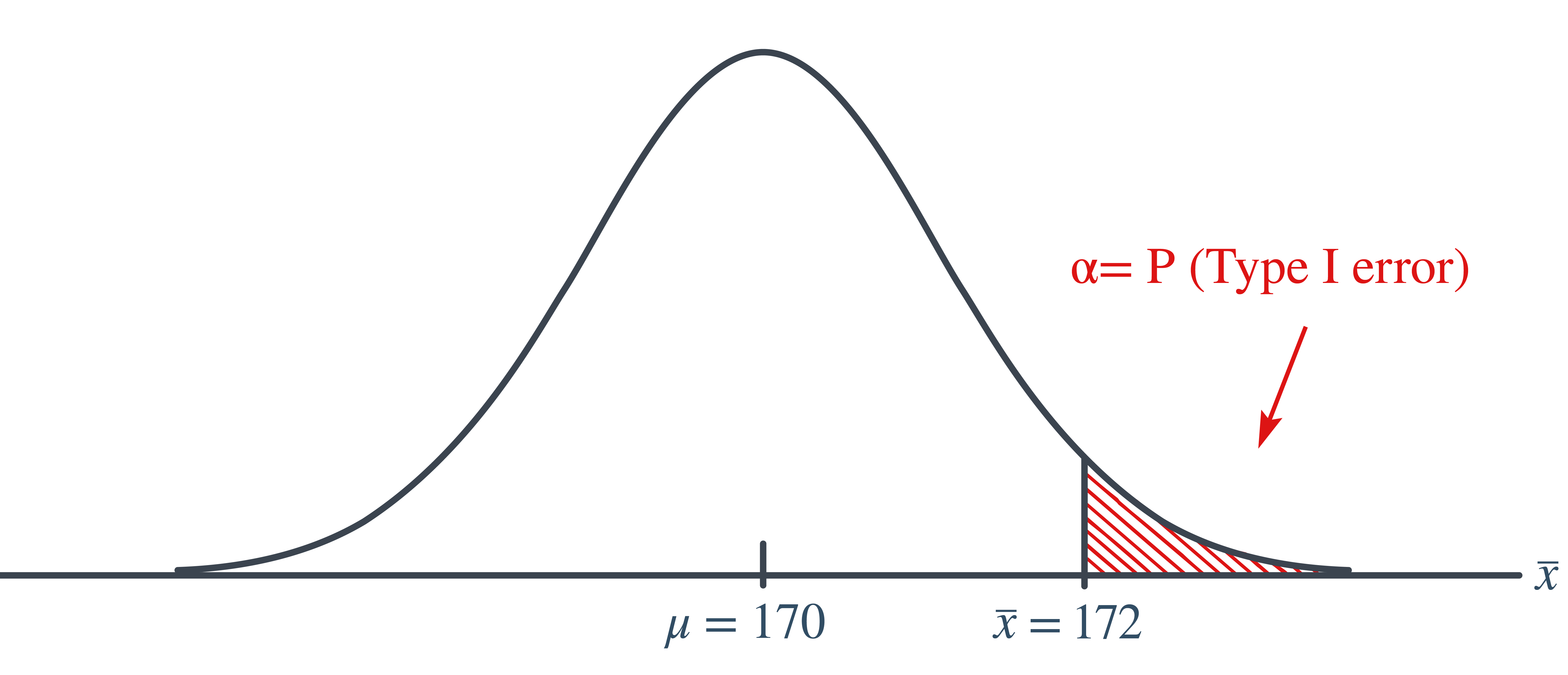
The Brinell hardness scale is one of several definitions used in the field of materials science to quantify the hardness of a piece of metal. The Brinell hardness measurement of a certain type of rebar used for reinforcing concrete and masonry structures was assumed to be normally distributed with a standard deviation of 10 kilograms of force per square millimeter. Using a random sample of \(n=25\) bars, an engineer is interested in performing the following hypothesis test:

• the null hypothesis \(H_0:\mu=170\)
• against the alternative hypothesis \(H_a: \mu>170\)

If the engineer decides to reject the null hypothesis if the sample mean is 172 or greater, that is, \(\bar{X}\ge 172\), what is the probability that the engineer commits a Type I error?

Solution

In this case, the engineer commits a Type I error if his observed sample mean falls in the rejection region, that is, if it is 172 or greater, when the true (unknown) population mean is indeed 170. Graphically, \(\alpha\), the engineer’s probability of committing a Type I error looks like this:

Fig 10.1

Now, we can calculate the engineer’s value of \(\alpha\) by making the transformation from a normal distribution with a mean of 170 and a standard deviation of 10 to that of \(Z\), the standard normal distribution using:

\[\begin{align*} Z=\frac{\bar{X}-\mu}{\frac{\sigma}{\sqrt{n}}} \end{align*}\]

Doing so, we get:

Fig 10.2

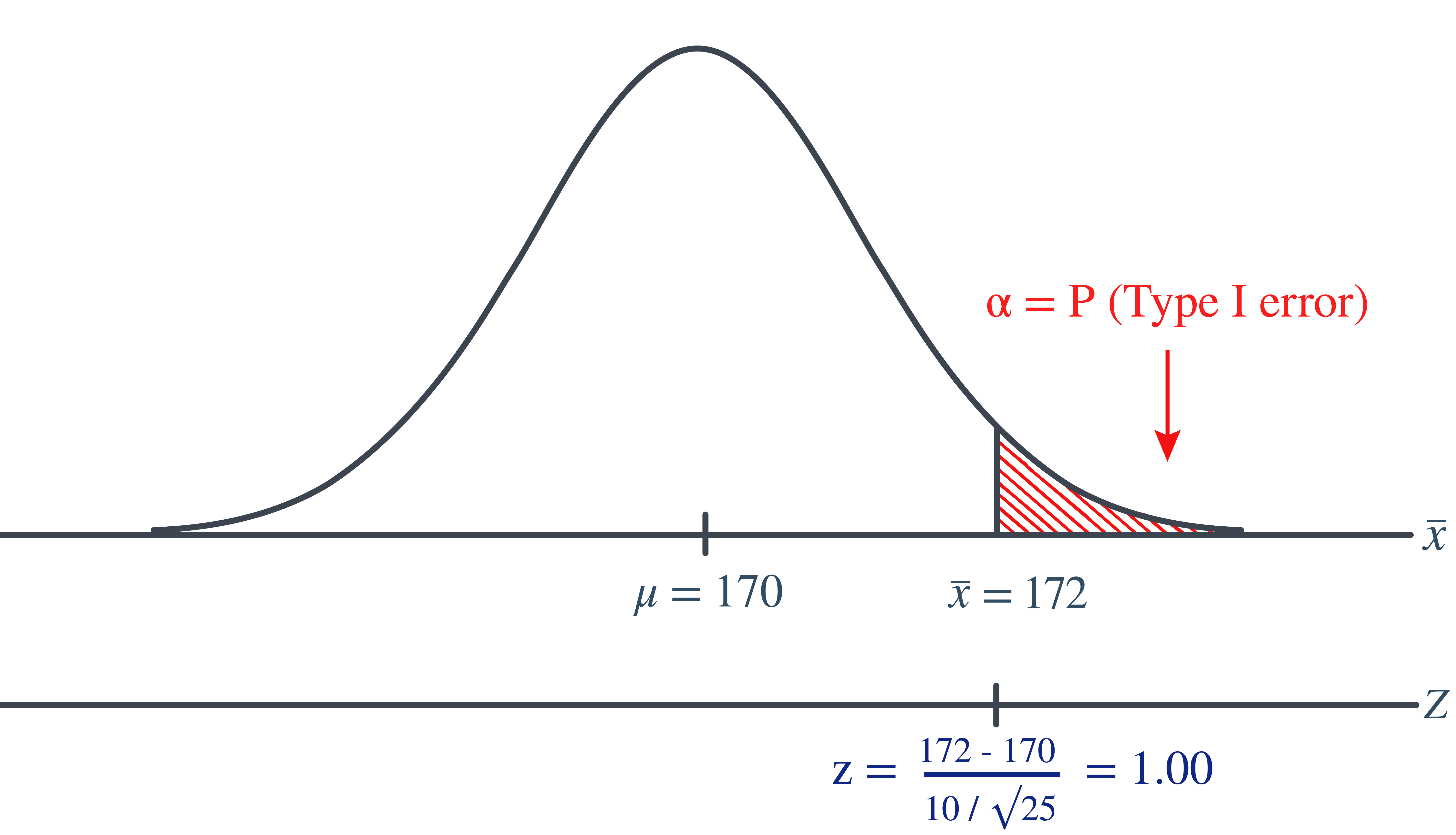
So, calculating the engineer’s probability of committing a Type I error reduces to making a normal probability calculation. The probability is 0.1587 as illustrated here:

\[\begin{align*} \alpha=P(\bar{X}\ge 172 \text{ if }\mu=170)=P(Z\ge 1.00)=0.1587 \end{align*}\]

A probability of 0.1587 is a bit high. We’ll learn in this lesson how the engineer could reduce his probability of committing a Type I error.

Part II
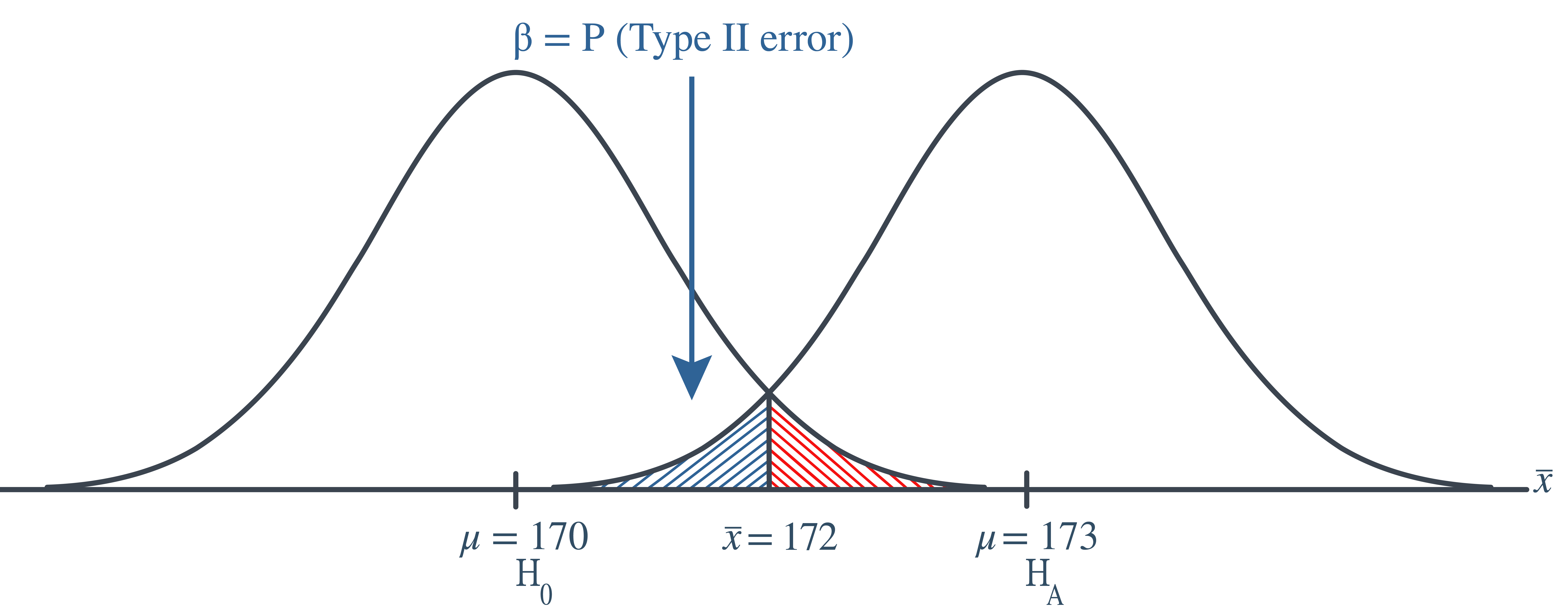
Continuing on with this example, if, unknown to the engineer, the true population mean were \(\mu=173\), what is the probability that the engineer commits a Type II error?

Solution

In this case, the engineer commits a Type II error if his observed sample mean does not fall in the rejection region, that is, if it is less than 172, when the true (unknown) population mean is 173. Graphically, \(\beta\), the engineer’s probability of committing a Type II error looks like this:

Fig 10.3

Again, we can calculate the engineer’s value of \(\beta\) by making the transformation from a normal distribution with a mean of 173 and a standard deviation of 10 to that of \(Z\), the standard normal distribution. Doing so, we get:

Fig 10.4

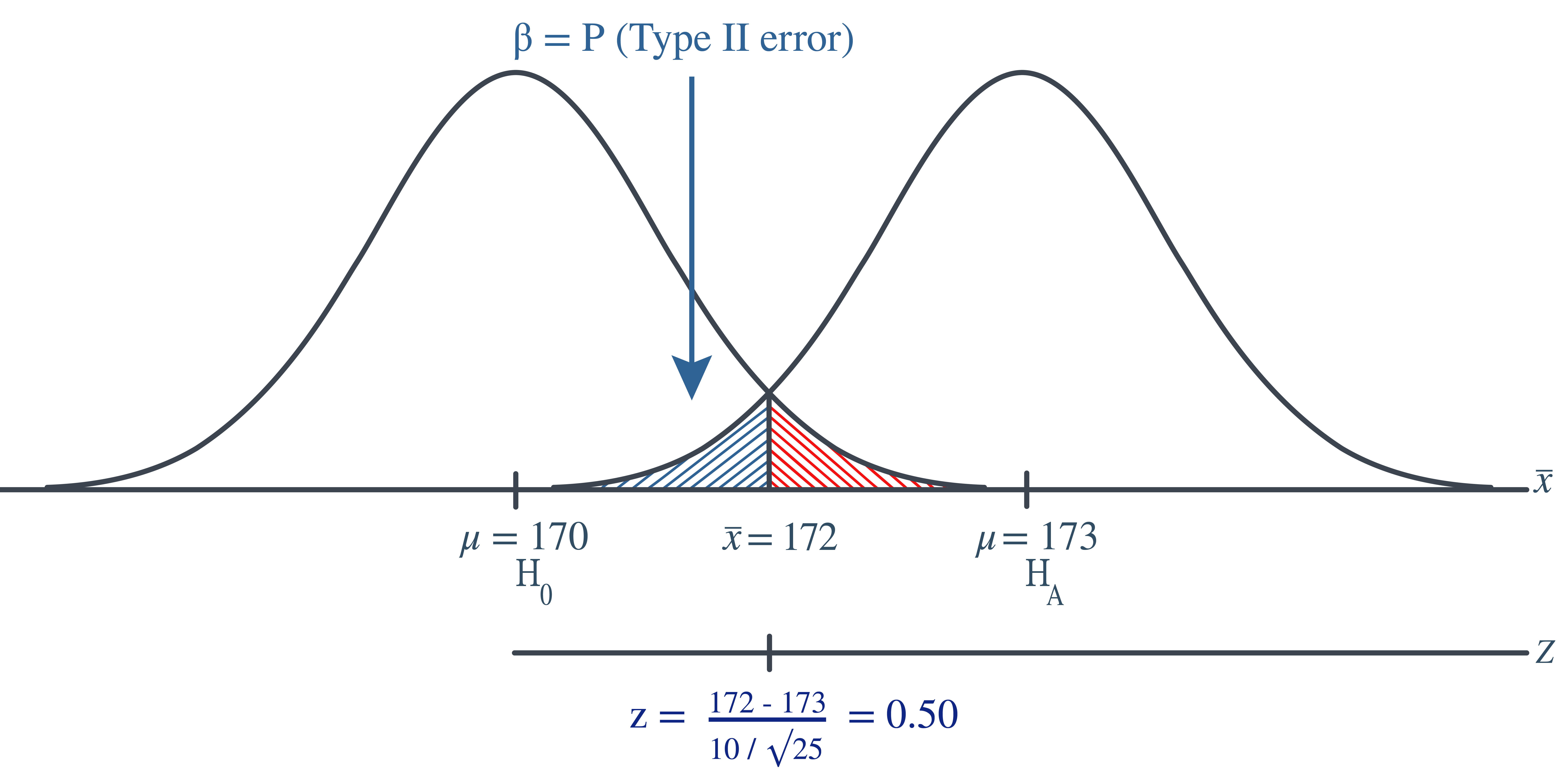
So, calculating the engineer’s probability of committing a Type II error again reduces to making a normal probability calculation. The probability is 0.3085 as illustrated here: \[\begin{align*} \beta=P(\bar{X}< 172 \text{ if }\mu=173)=P(Z<-0.50)=0.3085 \end{align*}\]

A probability of 0.3085 is a bit high. We’ll learn in this lesson how the engineer could reduce his probability of committing a Type II error.

If you think about it, considering the probability of committing a Type II error is quite similar to looking at a glass that is half empty. That is, rather than considering the probability that the engineer commits an error, perhaps we could consider the probability that the engineer makes the correct decision. Doing so involves calculating what is called the power of the hypothesis test.

Def. 10.1 (Power of a Test) The power of a hypothesis test is the probability of making the correct decision if the alternative hypothesis is true. That is, the power of a hypothesis test is the probability of rejecting the null hypothesis \(H_0\) when the alternative hypothesis \(H_a\) is the hypothesis that is true.

Let’s return to our engineer’s problem to see if we can instead look at the glass as being half full!

Example 10.5 Continuing with our previous example, if, unknown to the engineer, the true population mean was \(\mu=173\), what is the probability that the engineer makes the correct decision by rejecting the null hypothesis in favor of the alternative hypothesis?

Solution

In this case, the engineer makes the correct decision if his observed sample mean falls in the rejection region, that is, if it is greater than 172 when the true (unknown) population mean is 173. Graphically, the power of the engineer’s hypothesis test looks like this:

Fig 10.5

That makes the power of the engineer’s hypothesis test 0.6915 as illustrated here: \[\begin{align*} \text{Power}=P(\bar{X}\ge 172 \text{ if }\mu=173)=P(Z\ge -0.50)=0.6915 \end{align*}\] which of course could have alternatively been calculated by simply subtracting the probability of committing a Type II error from 1, as shown here: \[\begin{align*} \text{Power}=1-\beta=1-0.3085=0.6915 \end{align*}\]

At any rate, if the unknown population mean were 173, the engineer’s hypothesis test would be at least a bit better than flipping a fair coin, in which he’d have but a 50% chance of choosing the correct hypothesis. In this case, he has a 69.15% chance. He could still do a bit better.

In general, for every hypothesis test that we conduct, we’ll want to do the following:

1. Minimize the probability of committing a Type I error. That, is minimize \(\alpha=P(\text{Type I error})\). Typically, a significance level of \(\alpha\le 0.10\) is desired.

2. Maximize the power (at a value of the parameter under the alternative hypothesis that is scientifically meaningful). Typically, we desire power to be 0.80 or greater. Alternatively, we could minimize \(\beta=P(\text{Type II error})\) aiming for a type II error rate of 0.20 or less.

By the way, in the second point, what exactly does “at a value of the parameter under the alternative hypothesis that is scientifically meaningful” mean? Well, let’s suppose that a medical researcher is interested in testing the null hypothesis that the mean total blood cholesterol in a population of patients is 200 mg/dl against the alternative hypothesis that the mean total blood cholesterol is greater than 200 mg/dl. Well, the alternative hypothesis contains an infinite number of possible values of the mean. Under the alternative hypothesis, the mean of the population could be, among other values, 201, 202, or 210. Suppose the medical researcher rejected the null hypothesis because the mean was 201. Whoopdy-do…would that be a rocking conclusion? No, probably not. On the other hand, suppose the medical researcher rejected the null hypothesis, because the mean was 215. In that case, the mean is substantially different enough from the assumed mean under the null hypothesis, that we’d probably get excited about the result. In summary, in this example, we could probably all agree to consider a mean of 215 to be “scientifically meaningful,” whereas we could not do the same for a mean of 201.

Now, of course, all of this talk is a bit of gibberish, because we’d never really know whether the true unknown population mean was 201 or 215, otherwise, we wouldn’t have to be going through the process of conducting a hypothesis test about the mean. We can do something though. We can plan our scientific studies so that our hypothesis tests have enough power to reject the null hypothesis in favor of values of the parameter under the alternative hypothesis that is scientifically meaningful.

10.3.2 Power Functions

Let’s take a look at another example that involves calculating the power of a hypothesis test.

Example 10.6 Let \(X\) denote the IQ of a randomly selected adult American. Assume, a bit unrealistically, that \(X\) is normally distributed with unknown mean \(\mu\) and standard deviation 16. Take a random sample of \(n=16\) students, so that, after setting the probability of committing a Type I error at \(\alpha=0.05\), we can test the null hypothesis \(H_0:\mu=100\) against the alternative hypothesis that \(H_a: \mu>100\).

What is the power of the hypothesis test if the true population mean was \(\mu=108\)?

Solution

Setting \(\alpha\), the probability of committing a Type I error, to 0.05, implies that we should reject the null hypothesis when the test statistics \(Z\ge 1.645\), or equivalently, when the observed sample mean is 106.58 or greater:

Fig 10.6

because we transform the test statistic \(Z\) to the sample mean by way of: \[\begin{align*} & Z=\frac{\bar{X}-\mu}{\frac{\sigma}{\sqrt{n}}}, \qquad \Rightarrow \bar{X}=\mu+Z\frac{\sigma}{\sqrt{n}}\\ & \bar{X}=100+1.645\left(\frac{16}{\sqrt{16}}=106.58\right) \end{align*}\]

Now, that implies that the power, that is, the probability of rejecting the null hypothesis, when \(\mu=108\) is 0.6406 as calculated here (recalling that \(\Phi(z)\) is standard notation for the cumulative distribution function of the standard normal random variable):

\[\begin{align*} \text{Power}& =P(\bar{X}\ge 106.58 \text{ when }\mu=108)=P\left(Z\ge \frac{106.58-108}{\frac{16}{\sqrt{16}}}\right)\\ & P(Z\ge -0.36)=1-P(Z<-0.36)=1-\Phi(-0.36) \end{align*}\]

and illustrated here:

Fig 10.7

In summary, we have determined that we have (only) a 64.06% chance of rejecting the null hypothesis \(H_0:\mu=100\) in favor of the alternative hypothesis \(H_a: \mu>100\), if the true unknown population mean, is in reality \(\mu=108\).

Part II
Continuing with this example, what is the power of the hypothesis test if the true population mean were \(\mu=112\)?

Solution

Because we are setting \(\alpha\), the probability of committing a Type I error, to 0.05, we again reject the null hypothesis when the test statistic \(Z\ge 1.645\), or equivalently, when the observed sample mean is 106.58 or greater. That means that the probability of rejecting the null hypothesis, when \(\mu=112\), is 0.9131 as calculated here:

\[\begin{align*} \text{Power}&=P(\bar{X}\ge 106.58\text{ when }\mu=112)\\&=P\left(Z\ge \frac{106.58-112}{\frac{16}{\sqrt{16}}}\right) \\ &= P(Z\ge -1.36)\\&=1-P(Z<-1.36)\\&=1-\Phi(-1.36)\\&=1-0.0869=0.9131 \end{align*}\]

and illustrated here:

Fig 10.8

In summary, we have determined that we now have a 91.31% chance of rejecting the null hypothesis \(H_0: \mu=100\) in favor of the alternative hypothesis \(H_a: \mu>100\) if the true unknown population mean is in reality \(\mu=112\). Hmm…. it should make sense that the probability of rejecting the null hypothesis is larger for values of the mean, such as 112, that are far away from the assumed mean under the null hypothesis.

Part III
Again, continuing on with the previous example. What is the power of the hypothesis test if the true population mean were \(\mu=116\)?

Solution

Again, because we are setting \(\alpha\), the probability of committing a Type I error, to 0.05, we reject the null hypothesis when the test statistic \(Z\ge 1.645\), or equivalently, when the observed sample mean is 106.58 or greater. That means that the probability of rejecting the null hypothesis, when \(\mu=116\) is 0.9909 as calculated here:

\[\begin{align*} \text{Power}&=P(\bar{X}\ge 106.58\text{ when }\mu\\&=116) =P\left(Z\ge \dfrac{106.58-116}{\frac{16}{\sqrt{16}}}\right)\\ &= P(Z\ge -2.36)\\&=1-P(Z<-2.36)\\&= 1-\Phi(-2.36)\\&=1-0.0091=0.9909 \end{align*}\]

and illustrated here:

Fig 10.9

In summary, we have determined that, in this case, we have a 99.09% chance of rejecting the null hypothesis \(H_0: \mu=100\) in favor of the alternative hypothesis \(H_a: \mu>100\) if the true unknown population mean is in reality \(\mu=116\). The probability of rejecting the null hypothesis is the largest yet of those we calculated, because the mean, 116, is the farthest away from the assumed mean under the null hypothesis.

Are you growing weary of this? Let’s summarize a few things we’ve learned from engaging in this exercise:

1. First and foremost, my instructor can be tedious at times….. errrr, I mean, first and foremost, the power of a hypothesis test depends on the value of the parameter being investigated. In the above, example, the power of the hypothesis test depends on the value of the mean \(\mu\).

2. As the actual mean \(\mu\) moves further away from the value of the mean \(\mu=100\) under the null hypothesis, the power of the hypothesis test increases.

It’s that first point that leads us to what is called the power function of the hypothesis test. If you go back and take a look, you’ll see that in each case our calculation of the power involved a step that looks like this:

\[\begin{align*} \text{Power } =1 - \Phi (z) \end{align*}\]

That is, if we use the standard notation \(K(u)\) to denote the power function, as it depends on \(\mu\), we have: \[\begin{align*} K(\mu) = 1- \Phi \left( \frac{106.58 - \mu}{16 / \sqrt{16}} \right) \end{align*}\]

So, the reality is your instructor could have been a whole lot more tedious by calculating the power for every possible value of \(\mu\) under the alternative hypothesis! What we can do instead is create a plot of the power function, with the mean \(\mu\) on the horizontal axis and the power \(K(u)\) on the vertical axis. Doing so, we get a plot in this case that looks like this:

Fig 10.10

Now, what can we learn from this plot?

Well:

1. We can see that \(\alpha\) (the probability of a Type I error), \(\beta\) (the probability of a Type II error), and \(K(u)\) are all represented on a power function plot, as illustrated here:

Fig 10.11

2. We can see that the probability of a Type I error is \(\alpha=K(100)=0.05\), that is, the probability of rejecting the null hypothesis when the null hypothesis is true is 0.05.

3. We can see the power of a test \(K(u)\), as well as the probability of a Type II error \(\beta(u)\), for each possible value of \(\mu\).

4. We can see that \(\beta(u)=1-K(u)\) and vice versa, that is, \(K(u)=1-\beta(u)\).

5. And we can see graphically that, indeed, as the actual mean \(\mu\) moves further away from the null mean \(\mu=100\), the power of the hypothesis test increases.

Now, what would you suppose would happen to the power of our hypothesis test if we were to change our willingness to commit a Type I error? Would the power for a given value of \(\mu\) increase, decrease, or remain unchanged? Suppose, for example, that we wanted to set \(\alpha=0.01\) instead of \(\alpha=0.05\). Let’s return to our example to explore this question.

Example 10.7 Let \(X\) denote the IQ of a randomly selected adult American. Assume, a bit unrealistically, that \(X\) is normally distributed with unknown mean \(\mu\) and standard deviation 16. Take a random sample of \(n=16\) students, so that, after setting the probability of committing a Type I error at \(\alpha=0.01\), we can test the null hypothesis \(H_0:\mu=100\) against the alternative hypothesis that \(H_a: \mu>100\).

What is the power of the hypothesis test if the true population mean were \(\mu=108\)?

Solution

Setting \(\alpha\), the probability of committing a Type I error, to 0.01, implies that we should reject the null hypothesis when the test statistic \(Z\ge 2.326\), or equivalently, when the observed sample mean is 109.304 or greater:

Fig 10.12

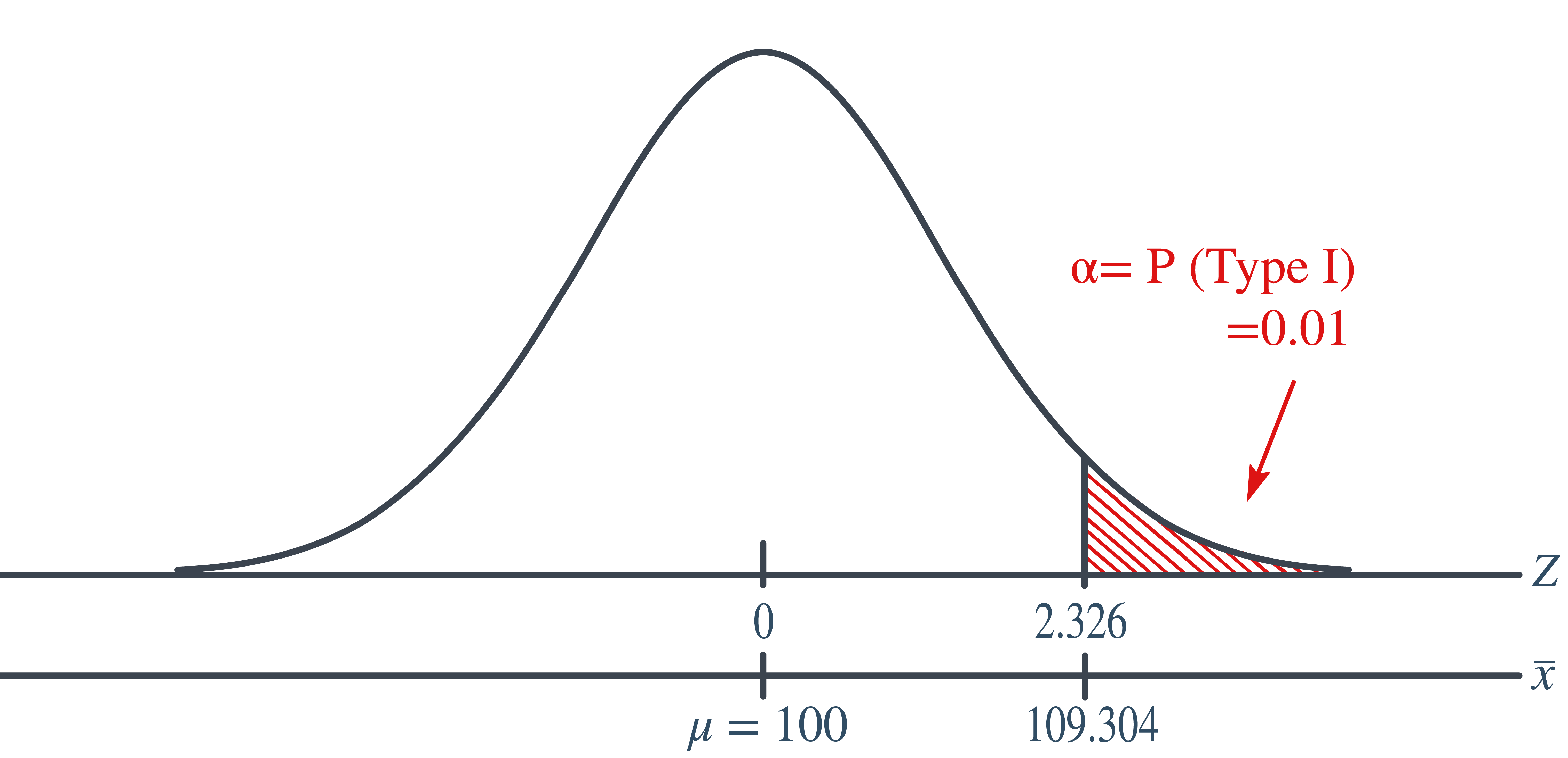
\[\begin{align*} \bar{x} = \mu + z \left( \frac{\sigma}{\sqrt{n}} \right) =100 + 2.326\left( \frac{16}{\sqrt{16}} \right)=109.304 \end{align*}\]

That means that the probability of rejecting the null hypothesis, when \(\mu=108\) is 0.3722 as calculated here:

\[\begin{align*} \text{Power}&=P(\bar{X}\ge 109.304 \text{ when }\mu=108)=P\left(Z\ge \frac{109.304-108}{\frac{16}{\sqrt{16}}}\right)\\ & = P(Z\ge 0.326)=1-P(Z<0.326)=1-\Phi(0.326)\\ & = 1-0.6278=0.3722 \end{align*}\]

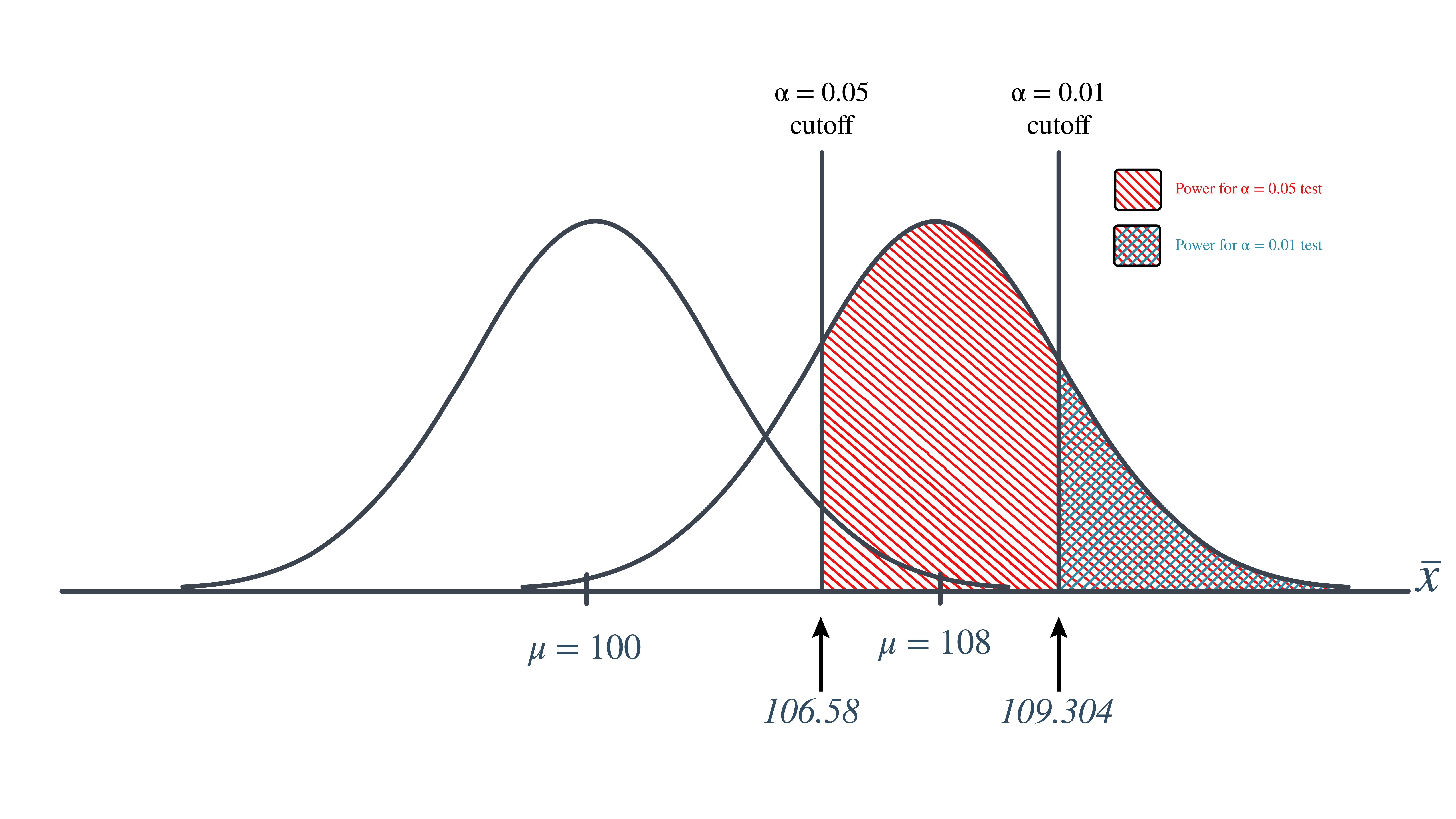
So, the power when \(\mu=108\) and \(\alpha=0.01\) is smaller (0.3722) than the power when \(\mu=108\) and \(\alpha=0.05\) (0.6406)! Perhaps we can see this graphically:

Fig 10.13

By the way, we could again alternatively look at the glass as being half-empty. In that case, the probability of a Type II error when \(\mu=108\) and \(\alpha=0.01\) is \(1-0.326=0.6278\). In this case, the probability of a Type II error is greater than the probability of a Type II error when \(\mu=108\) and \(\alpha=0.05\).

All of this can be seen graphically by plotting the two power functions, one where \(\alpha=0.01\) and the other where \(\alpha=0.05\), simultaneously. Doing so, we get a plot that looks like this:

This last example illustrates that providing the sample size \(n\) remains unchanged, a decrease in \(\alpha\) causes an increase in \(\beta\), and at least theoretically, if not practically, a decrease in \(\beta\) causes an increase in \(\alpha\). It turns out that the only way that \(\alpha\) and \(\beta\) can be decreased simultaneously is by increasing the sample size \(n\).

10.3.3 Calculating Sample Size

Before we learn how to calculate the sample size that is necessary to achieve a hypothesis test with a certain power, it might behoove us to understand the effect that sample size has on power. Let’s investigate by returning to our IQ example.

Example 10.8 Let \(X\) denote the IQ of a randomly selected adult American. Assume, a bit unrealistically again, that \(X\) is normally distributed with unknown mean \(\mu\) and (a strangely known) standard deviation of 16. This time, instead of taking a random sample of \(n=16\) students, let’s increase the sample size to \(n=64\). And, while setting the probability of committing a Type I error to \(\alpha=0.05\), test the null hypothesis \(H_0:\mu=100\) against the alternative hypothesis that \(H_a:\mu>100\).

What is the power of the hypothesis test when \(\mu=108\), \(\mu=112\), and \(\mu=116\)?

Solution

Setting \(\alpha\), the probability of committing a Type I error, to 0.05, implies that we should reject the null hypothesis when the test statistic \(Z\ge 1.645\), or equivalently, when the observed sample mean is 103.29 or greater:

Fig 10.14

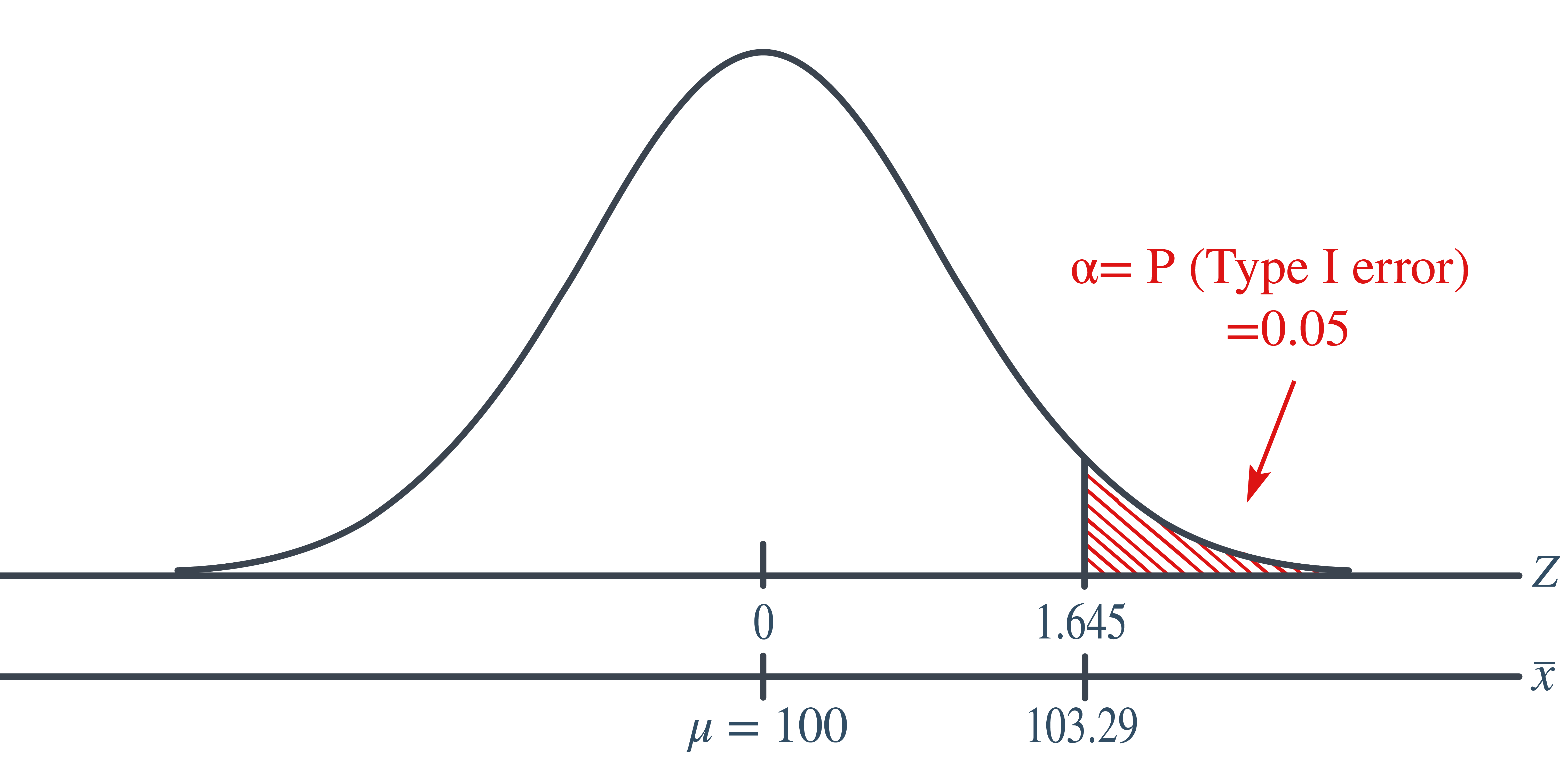
because:

\[\begin{align*} \bar{x} &= \mu + z \left(\dfrac{\sigma}{\sqrt{n}} \right)\\ &= 100 +1.645\left(\dfrac{16}{\sqrt{64}} \right) = 103.29 \end{align*}\]

Therefore, the power function \(K(\mu)\), when \(\mu>100\) is the true value, is:

\[\begin{align*} K(\mu) &= P(\bar{X} \ge 103.29 | \mu)\\ &= P \left(Z \ge \dfrac{103.29 - \mu}{16 / \sqrt{64}} \right)\\ &= 1 - \Phi \left(\dfrac{103.29 - \mu}{2} \right) \end{align*}\]

Therefore, the probability of rejecting the null hypothesis at the \(\alpha=0.05\) level when \(\mu=108\) is 0.9907, as calculated here:

\[\begin{align*} K(108) &= 1 - \Phi \left( \dfrac{103.29-108}{2} \right) = 1- \Phi(-2.355) = 0.9907 \end{align*}\]

And, the probability of rejecting the null hypothesis at the \(\alpha=0.05\) level when \(\mu=112\) is greater than 0.9999, as calculated here:

\[\begin{align*} K(112) &= 1 - \Phi \left( \dfrac{103.29-112}{2} \right)\\ &= 1- \Phi(-4.355)\\ &= 0.9999\ldots \end{align*}\]

And, the probability of rejecting the null hypothesis at the \(\alpha=0.05\) level when \(\mu=116\) is greater than 0.999999, as calculated here:

\[\begin{align*} K(116) &= 1 - \Phi \left( \dfrac{103.29-116}{2} \right)\\ &= 1- \Phi(-6.355)\\ &= 0.999999... \end{align*}\]

In summary, in the various examples throughout this lesson, we have calculated the power of testing \(H_0:\mu=100\) against \(H_a:\mu>100\) for two sample sizes (\(n=16\) and \(n=64\)) and for three possible values of the mean ( \(\mu=108\), \(\mu=112\), and \(\mu=116\)). Here’s a summary of our power calculations:

Power	\(K(108)\)	\(K(112)\)	\(K(116)\)
\(n=16\)	0.6406	0.9131	0.9909
\(n=64\)	0.9907	0.9999…	0.999999…

As you can see, our work suggests that for a given value of the mean \(\mu\) under the alternative hypothesis, the larger the sample size \(n\), the greater the power \(K(u)\). Perhaps there is no better way to see this than graphically by plotting the two power functions simultaneously, one when \(n=16\) and the other when \(n=64\):

Fig 10.15

As this plot suggests, if we are interested in increasing our chance of rejecting the null hypothesis when the alternative hypothesis is true, we can do so by increasing our sample size \(n\). This benefit is perhaps even greatest for values of the mean that are close to the value of the mean assumed under the null hypothesis. Let’s take a look at two examples that illustrate the kind of sample size calculation we can make to ensure our hypothesis test has sufficient power.

Example 10.9 Let \(X\) denote the crop yield of corn measured in the number of bushels per acre. Assume (unrealistically) that \(X\) is normally distributed with unknown mean \(\mu\) and standard deviation \(\sigma=6\). An agricultural researcher is working to increase the current average yield from 40 bushels per acre. Therefore, he is interested in testing, at the \(\alpha=0.05\) level, the null hypothesis \(H_0:\mu=40\) against the alternative hypothesis that \(H_a:\mu>40\). Find the sample size \(n\) that is necessary to achieve 0.90 power at the alternative \(\mu=45\).

Solution

As is always the case, we need to start by finding a threshold value \(c\), such that if the sample mean is larger than \(c\), we’ll reject the null hypothesis:

Fig 10.16

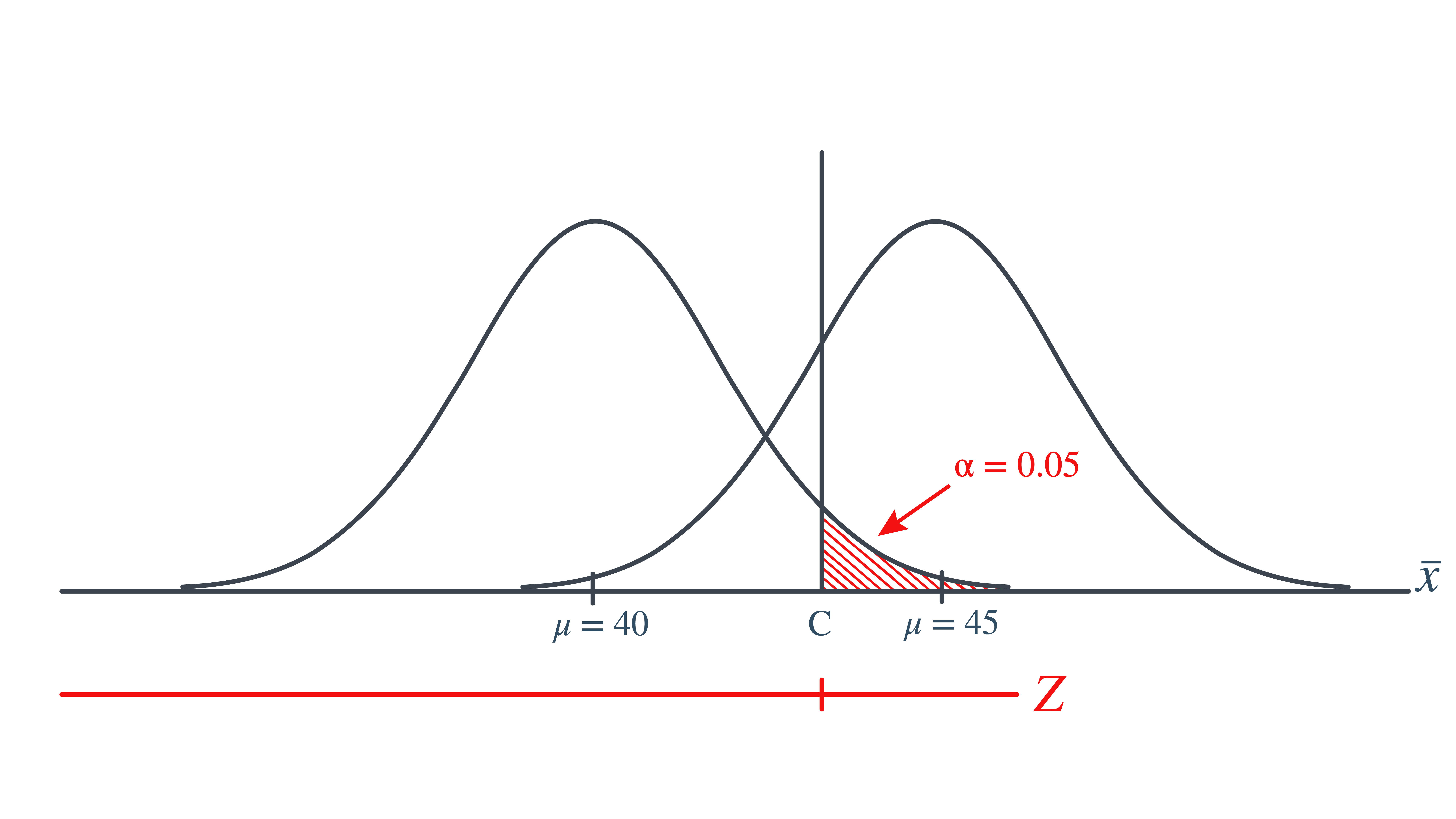
That is, in order for our hypothesis test to be conducted at the \(\alpha=0.05\) level, the following statement must hold (using our typical \(Z\) transformation):

\[\begin{align} c = 40 + 1.645 \left( \dfrac{6}{\sqrt{n}} \right) \end{align}\]

But, that’s not the only condition that \(c\) must meet, because \(c\) also needs to be defined to ensure that our power is 0.90 or, alternatively, that the probability of a Type II error is 0.10. That would happen if there was a 10% chance that our test statistic fell short of \(c\) when \(\mu=45\), as the following drawing illustrates in blue:

Fig 10.17

This illustration suggests that in order for our hypothesis test to have 0.90 power, the following statement must hold (using our usual \(Z\) transformation):

\[\begin{align} c = 45 - 1.28 \left( \dfrac{6}{\sqrt{n}} \right) \end{align}\]

Aha! We have two ((1) and (2)) equations and two unknowns! All we need to do is equate the equations and solve for \(n\). Doing so, we get:

\[\begin{align*} & 40+1.645\left(\frac{6}{\sqrt{n}}\right)=45-1.28\left(\frac{6}{\sqrt{n}}\right)\\ & \Rightarrow 5=(1.645+1.28)\left(\frac{6}{\sqrt{n}}\right), \qquad \Rightarrow 5=\frac{17.55}{\sqrt{n}}, \qquad n=(3.51)^2=12.3201\approx 13 \end{align*}\]

Now that we know we will set \(n=13\), we can solve for our threshold value \(c\):

\[\begin{align*} c = 40 + 1.645 \left( \dfrac{6}{\sqrt{13}} \right)=42.737 \end{align*}\]

So, in summary, if the agricultural researcher collects data on \(n=13\) corn plots, and rejects his null hypothesis \(H_0:\mu=40\) if the average crop yield of the 13 plots is greater than 42.737 bushels per acre, he will have a 5% chance of committing a Type I error and a 10% chance of committing a Type II error if the population mean \(\mu\) were actually 45 bushels per acre.

Part II

Consider \(p\), the true proportion of voters who favor a particular political candidate. A pollster is interested in testing at the \(\alpha=0.01\) level, the null hypothesis \(H_0:p=0.5\) against the alternative hypothesis that \(H_a:p>0.5\). Find the sample size \(n\) that is necessary to achieve 0.80 power at the alternative \(p=0.55\).

Solution

In this case, because we are interested in performing a hypothesis test about a population proportion \(p\), we use the \(Z\)-statistic:

\[\begin{align*} Z = \dfrac{\hat{p}-p_0}{\sqrt{\frac{p_0(1-p_0)}{n}}} \end{align*}\]

Again, we start by finding a threshold value \(c\), such that if the observed sample proportion is larger than \(c\), we’ll reject the null hypothesis:

Fig 10.18

That is, in order for our hypothesis test to be conducted at the \(\alpha=0.01\) level, the following statement must hold:

\[\begin{align} c = 0.5 + 2.326 \sqrt{ \dfrac{(0.5)(0.5)}{n}} \end{align}\]

But, again, that’s not the only condition that c must meet, because \(c\) also needs to be defined to ensure that our power is 0.80 or, alternatively, that the probability of a Type II error is 0.20. That would happen if there was a 20% chance that our test statistic fell short of \(c\) when \(p=0.55\), as the following drawing illustrates in blue:

Fig 10.19

This illustration suggests that in order for our hypothesis test to have 0.80 power, the following statement must hold:

\[\begin{align} c = 0.55 - 0.842 \sqrt{ \dfrac{(0.55)(0.45)}{n}} \end{align}\]

Again, we have two ((3) and (4)) equations and two unknowns! All we need to do is equate the equations, and solve for \(n\). Doing so, we get:

\[\begin{align*} 0.5+2.326\sqrt{\dfrac{0.5(0.5)}{n}}&=0.55-0.842\sqrt{\dfrac{0.55(0.45)}{n}} \\ 2.326\dfrac{\sqrt{0.25}}{\sqrt{n}}+0.842\dfrac{\sqrt{0.2475}}{\sqrt{n}}&=0.55-0.5 \\ \dfrac{1}{\sqrt{n}}(1.5818897)&=0.05 \qquad\\ &\Rightarrow n\approx \left(\dfrac{1.5818897}{0.05}\right)^2\\ &= 1000.95 \approx 1001 \end{align*}\]

Now that we know we will set \(n=1001\), we can solve for our threshold value \(c\):

\[\begin{align*} c = 0.5 + 2.326 \sqrt{\dfrac{(0.5)(0.5)}{1001}}= 0.5367 \end{align*}\]

So, in summary, if the pollster collects data on \(n=1001\) voters, and rejects his null hypothesis \(H_0:p=0.5\) if the proportion of sampled voters who favor the political candidate is greater than 0.5367, he will have a 1% chance of committing a Type I error and a 20% chance of committing a Type II error if the population proportion \(p\) were actually 0.55.

Incidentally, we can always check our work! Conducting the survey and subsequent hypothesis test as described above, the probability of committing a Type I error is:

\[\begin{align*} \alpha= P(\hat{p} >0.5367 \text { if } p = 0.50) = P(Z > 2.3257) = 0.01 \end{align*}\]

and the probability of committing a Type II error is:

\[\begin{align*} \beta = P(\hat{p} <0.5367 \text { if } p = 0.55) = P(Z < -0.846) = 0.199 \end{align*}\]

just as the pollster had desired.

We’ve illustrated several sample size calculations. Now, let’s summarize the information that goes into a sample size calculation. In order to determine a sample size for a given hypothesis test, you need to specify:

1. The desired \(\alpha\) level, that is, your willingness to commit a Type I error.

2. The desired power or, equivalently, the desired \(\beta\) level, that is, your willingness to commit a Type II error.

3. A meaningful difference from the value of the parameter that is specified in the null hypothesis.

4. The standard deviation of the sample statistic or, at least, an estimate of the standard deviation (the “standard error”) of the sample statistic.

10.4 Approximate Wald Test

In the hypothesis tests we have developed so far, we need to find a test statistic and know the distribution of the test statistic under the null hypothesis. However, how do we choose the test statistic? Can we always find the distribution of the test statistic? Is the test statistic based on a statistic (or estimator) that has desirable properties?

Based on what we learned so far in this class, we know the MLE has desirable properties, especially under certain conditions. We present in this lesson the Wald test. It is a test generally applicable with using the MLE and relies on the asymptotic normality of the MLE.

10.4.1 The Step Up

As we have noted before, if we consider each data point \(x_i\) as a random variable, with \[\begin{align*} x_i \sim f_X(x|\theta) \end{align*}\] then any function of these data points is a random variable. In particular, the MLE \(\hat{\theta}=\text{argmax}(L(\theta))\) is a function of the data, and so it is a random variable. In some simple cases, we can work out the distribution of \(\hat{\theta}\) directly, but in many cases we cannot. Fortunately, there is a result that, for any MLE, regardless of the distribution \(f_X\) that the data come from, the MLE is normally-distributed.

For single parameter models, the result is as follows:

If \(L(\theta|x_1,x_2,\ldots,x_n)\) is the likelihood function and \(\hat{\theta}=\text{argmax}(L(\theta))\) is the MLE, then, as \(n\rightarrow \infty\), \[ \hat{\theta}_{ML}\sim N\left(\theta_{\text{true}},1/I(\hat{\theta}_{ML})\right)\] where \(I(\theta)\) is the “Fisher Information”, defined by \[I(\theta) = -E_x\left[\frac{\partial^2}{\partial \theta^2}\ell(\theta)\right]\] where \(\ell(\theta)=log(L(\theta))\) and the expectation is taken over all \(x_1,x_2,\ldots,x_n\).

In the multivariate case, where there are two or more parameters to be estimated, \(\boldsymbol\theta=(\theta_1,\theta_2,\ldots,\theta_p)\) is the vector of \(p\) parameters to be estimated and the asymptotic distribution is as follows. as \(n\rightarrow \infty\), \[ \hat{\boldsymbol\theta}_{ML}\sim N\left(\boldsymbol\theta_{\text{true}},\mathbf{I}^{-1}(\hat{\boldsymbol\theta}_{ML})\right)\] where \(\mathbf{I}(\boldsymbol\theta)\) is the “Fisher Information Matrix”, defined by \[\mathbf{I}(\boldsymbol\theta) = \left[\begin{array}{cccc} -E_x\left[\frac{\partial^2}{\partial \theta_1^2}\ell(\theta)\right] & -E_x\left[\frac{\partial^2}{\partial \theta_1\partial\theta_2}\ell(\theta)\right] & \cdots & -E_x\left[\frac{\partial^2}{\partial \theta_1\partial\theta_p}\ell(\theta)\right]\\ -E_x\left[\frac{\partial^2}{\partial \theta_2\partial\theta_1}\ell(\theta)\right] & -E_x\left[\frac{\partial^2}{\partial\theta_2^2}\ell(\theta)\right] & \cdots & -E_x\left[\frac{\partial^2}{\partial \theta_2\partial\theta_p}\ell(\theta)\right] \\ \vdots & \vdots & & \vdots \\ -E_x\left[\frac{\partial^2}{\partial \theta_p\partial\theta_1}\ell(\theta)\right] & -E_x\left[\frac{\partial^2}{\partial \theta_p\partial\theta_2}\ell(\theta)\right] & \cdots & -E_x\left[\frac{\partial^2}{\partial \theta_p^2}\ell(\theta)\right] \end{array}\right] \] where again \(\ell(\theta)=log(L(\theta))\) and the expectation is taken over all \(x_1,x_2,\ldots,x_n\). This result details the approximate joint distribution of the MLEs of all of the parameters. For many situations (including for most hypothesis tests), a more useful result is the resulting marginal distribution of each individual MLE. If the \(k\)-th parameter is \(\theta_k\), and the MLE for this parameter is \(\hat{\theta}_k\), then a direct result of the joint distribution above is that the marginal distribution of \(\hat{\theta}_k\) is asymptotically approximately Gaussian, with \[ \hat{\theta}_k \approx N(\theta_{k,true},\mathbf{I}^{-1}(\hat{\boldsymbol\theta})_{[k,k]})\] That is, the MLE \(\hat{\theta}_k\) is approximately univariate normally distributed, with mean the true parameter \(\theta_k\) and variance equal to the \(k\)-th diagonal entry of the inverse \(\mathbf{I}^{-1}(\hat{\boldsymbol\theta})\) of the Fisher information matrix.

We can use the asymptotic approximate Gaussian distribution of MLEs described previously to construct test statistics that are useful for testing \(H_0:\theta_k=c\) versus \(H_A:\theta_k \neq c\).

Since we know that \[ \hat{\theta}_k \approx N(\theta_{k,true},\mathbf{I}^{-1}(\hat{\boldsymbol\theta})_{[k,k]})\] if the null hypothesis is that \(\theta_k=c\), then under \(H_0\), the distribution of the MLE is \[ \hat{\theta}_k \approx N(c,\mathbf{I}^{-1}(\hat{\boldsymbol\theta})_{[k,k]})\]

Following our notation above, we have a test statistic (we’re calling it \(\hat{\theta}_k\) here, while in the general description above we called it \(T^*\)), and we know the (approximate) distribution of this statistic (\(T\sim N(c,\mathbf{I}^{-1}(\hat{\boldsymbol\theta})_{[k,k]})\) under the null hypothesis. A p-value would then be \[p=P(|T|\geq |\hat{\theta}_k|),\text{ where } T\sim N(c,\mathbf{I}^{-1}(\hat{\boldsymbol\theta})_{[k,k]})\] We could simplify this a little. If we first define the \(k\)-th standard error \(se_k\) as \[se_k=\sqrt{\mathbf{I}^{-1}(\hat{\boldsymbol\theta})_{[k,k]}}\] then by subtracting the mean and dividing by \(se_k\) we obtain \[ Z^*=\frac{\hat{\theta}_k-c}{se_k}\sim N(0,1)\] where \(Z^*\approx N(0,1)\). The p-value (probability of observing a more extreme value if the null hypothesis is true) can then be written as \[p=P(|Z|>|Z^*|)=P(Z<-|Z^*|)+P(Z>|Z^*|)\] which, by the symmetry of a standard normal distribution, is equal to \[p=2*P(Z\leq -|Z^*|)=2\Phi(-|Z^*|)\] This sort of test, based on the asymptotic approximate gaussian distribution of the MLE, is called a Wald test.

10.4.2 A Recipe for Wald Tests

To summarize the above results, if \(x_i \sim f_X(x|\boldsymbol\theta)\) are independent random variables, and we want to test the null hypothesis that \(H_0:\theta_k=c\) versus the alternate that \(H_A:\theta_k \neq c\), then a Wald test of this hypothesis is conducted by the following:

1. We first find the MLE of all parameters \(\hat{\boldsymbol\theta}\) in the model, and the corresponding Fisher information \(\mathbf{I}(\hat{\boldsymbol\theta})\).
2. We then find the \(k\)-th standard error \(se_k=\sqrt{\mathbf{I}^{-1}(\hat{\boldsymbol\theta})_{[k,k]}}\) and construct the test statistic \[Z^*=\frac{\hat{\theta}_k-c}{se_k}\]
3. A Wald p-value for this test is then \[p=2*P(Z\leq -|Z^*|)=2\Phi(-|Z^*|)\]
4. If the above calculated p-value is \(p<\alpha\) then we reject \(H_0\) and accept \(H_A\). If the above calculated p-value is \(p>\alpha\) then we fail to reject \(H_0\) and conclude that there is not sufficient evidence to disprove \(H_0\).

10.4.3 Examples of Hypothesis Testing

In this section, we present an example of hypothesis testing, focusing on Wald tests for MLEs.

Example 10.10 (A Bernoulli/Binomial Example of Hypothesis Testing) Assume that a casino has a game of chance that has a published probability of winning of 0.25. Assume that a person plays the game of chance 20 times, and wins the game exactly once. From that experience, is there enough evidence to conclude that the game of chance does not, in fact, have a win rate of 25%?

To frame this as a hypothesis test, we first need a parametric statistical model for the observed data. We assume that each of the 20 games played is independent of each other, and each has a probability \(p\) of resulting in a “win”. So \[ x_i \sim Bern(p),\ \ i=1,2,\ldots,20\] With the actual observed data including exactly one win (without loss of generality, let \(x_1=1\)) and 19 losses (let \(x_2=0,\ x_3=0,\ \ldots,x_20=0\)).

Our goal is to determine if we have enough evidence to conclude that the win rate is NOT 25%. We thus specify a null hypothesis that \[H_0:p=0.25\] with the corresponding alternative hypothesis that \(H_A:p\neq 0.25\). We will consider a Wald test of this hypothesis. Before constructing the test, we set the level of the test to be \(\alpha=0.05\), so we are willing to conclude that the null hypothesis is false if the probability (under \(H_0\)) of observing the test statistic we will construct is 5% or less.

An Analytic Wald Hypothesis Test for Bernoulli Data

We first illustrate constructing a Wald hypothesis test analytically, following the procedure outlined above.

1. We first find the MLE and Fisher Information of the parameter \(p\).

   From previous examples in class, we know that the MLE is \[\hat{p}=\frac{\sum_{i=1}^{20} x_i}{20}=\frac{1}{20}=0.05\] and that the Fisher Information is \[I(\hat{p})=-E_x(\ell''(\hat{p})))=\frac{20}{\hat{p}(1-\hat{p})}=\frac{20}{.05(.95)}=421.0526\]

2. We then find the standard error \[ se=\sqrt{1/I(\hat{p})}=\sqrt{1/421.0526}=0.0487\] and construct the Wald test statistic \[ Z^*=\frac{\hat{p}-0.25}{se}=\frac{0.05-0.25}{0.0487}=-4.104\]

3. We then find the p-value of this test statistic under the null hypothesis \[pval=2*P(Z\leq-|Z^*|)=2*P(Z\leq-4.104)\] which we evaluate in R:

    phat=.05
    I=421.0526
    se=sqrt(1/I)
    Z.star=(.05-.25)/se
    pval=2*pnorm(-abs(Z.star))
    pval

   [1] 4.062198e-05

   which results in a p-value of 0.0000406

4. As this p-value is much smaller than the level \(\alpha=0.05\), we reject \(H_0:p=0.25\) and conclude that the win rate for the game of chance is very unlikely to be the stated rate of .025.

A Numeric Wald Hypothesis Test

We now construct the same hypothesis test using numeric maximum likelihood analysis. We first enter the data

x=c(1,0,0,0,0,0,0,0,0,0,0,0,0,0,0,0,0,0,0,0)
n=length(x)

We then write a function to evaluate the negative log likelihood and find the MLE and Fisher Information using optim.

## negative log likelihood function
nll.bern=function(p,x){
    -sum(log(dbinom(x,size=1,prob=p)))
}
## run optim
out=optim(.5,nll.bern,x=x,hessian=TRUE)
## save MLE
p.hat=out$par
## save Fisher Information
I=out$hessian

Using these, we find our standard error and then the Wald Test Statistic

se=sqrt(1/I)
## get Wald test statistic
T.star=(p.hat-0.25)/se
T.star

          [,1]
[1,] -4.105474

And then the p-value is

pval=2*pnorm(-abs(T.star),mean=0,sd=1)
pval

             [,1]
[1,] 4.034858e-05

which again is much smaller than the level \(\alpha=0.05\), we reject \(H_0:p=0.25\) and conclude that the win rate for the game of chance is very unlikely to be the stated rate of .025.

10.5 Summary

In this lesson we deepened our hypothesis‑testing toolkit by explicitly connecting confidence intervals to their companion tests, examining the tug‑of‑war between Type I and II errors through the lens of power, and meeting the Wald test—a versatile large‑sample method built on maximum‑likelihood estimators. You will also see how design choices such as sample size, significance level (), and effect size interact when planning a study.

Key takeaways:

• A two‑sided null value that lies outside its corresponding confidence interval is automatically rejected by the matching test.
• Increasing sample size tightens confidence intervals and boosts power without altering .
• Power calculations let you choose a sample size that has a high probability of detecting effects that matter.
• The Wald test furnishes an approximate ‑test for any parameter whose MLE is asymptotically normal, extending hypothesis‑testing tools to models where classical formulas are unwieldy.