Alert - Under construction. This is a development site only.
7Asymptotic Distribution of MLE (Part I)
MLEs
Asymptotic Confidence Intervals
Numerical Approximations
Bootstrap
Overview
Let’s revisit maximum likelihood estimators (MLEs) to explore their asymptotic properties and their application in constructing confidence intervals. This lesson introduces the theoretical foundations of MLEs, including their consistency, equivariance, and asymptotic normality under regularity conditions. You will learn to derive the Fisher Information for single and multiple parameter models and use it to construct asymptotic confidence intervals. The lesson also covers numerical approximations of these intervals using R’s optim function and introduces the bootstrap method—both parametric and nonparametric—for estimating confidence intervals when analytical solutions are infeasible. Additionally, you will explore the Delta method and bootstrap approaches for inference on transformations of parameters. Through examples involving Bernoulli, exponential, normal, geometric, t, and Pareto distributions, you will gain practical skills in applying these techniques, preparing you for advanced statistical inference. Let us dive in.
Objectives
Upon completion of this lesson, you should be able to:
7.1 Properties of MLEs
Maximum likelihood estimation is popular because there are a number of provable properties that apply to ANY MLE!
The following result holds for any MLE, subject to some “regularity conditions”. The regularity conditions include
The underlying probability function, \(f(x|\theta)\), is “smooth”.
The estimator, \(\hat{\theta}_{mle}\), is NOT on the edge of allowable values. For example, the MLE is not in the support.
We will not show the full list of conditions nor proofs of the following properties. You can find them in the Wasserman text, chapter 9.13.
Property 1: The estimator, \(\hat{\theta}_{mle}\) is consistent.
This means that as the sample size \(n\) approaches infinity, \(\hat{\theta}_{mle}\) approaches the true \(\theta\). A corollary to this is as \(n\) approaches infinity, \(E(\hat{\theta}_{mle})\) approaches the true \(\theta\).
Property 2: The estimator, \(\hat{\theta}_{mle}\), is equivariant.
An estimator, \(\hat{\theta}\), is the MLE of \(\theta\), and \(g(\theta)\) is an invertible function, then the MLE of \(\tau=g(\theta)\) is \(\hat{\tau}=g(\hat{\theta})\).
This means that MLE of a function of a parameter is the function of the MLE of the parameter, as long as the function is invertible.
Example 7.1 Let \(X_i\sim N(\mu, \sigma^2)\). That is, let \(X_1, X_2, \ldots, X_n\) be iid Normal random variables with mean \(\mu\) and variance \(\sigma^2\). We know that \(\hat{\mu}=\bar{x}\) and \(\hat{\sigma}^2=\frac{1}{n}\sum_{i=1}^n(x_i-\bar{x})^2\) are the MLEs of \(\mu\) and \(\sigma^2\), respectfully. What is the MLE of the standard deviation, \(\sigma\)?
Solution
We know \(\sigma=g(\sigma^2)=\sqrt{\sigma^2}\). Therefore, based on the equivariant property, the MLE of \(\sigma\) is: \[\begin{align*}
\hat{\sigma}_{mle}=\sqrt{\hat{\sigma}^2_{mle}}=\sqrt{\frac{1}{n}\sum_{i=1}^n (x_i-\bar{x})^2}
\end{align*}\]
Example 7.2 Let \(X_i\sim Bin(5, p)\), for \(i=1, \ldots, n\). What is the MLE of the odds ratio, \(\text{OR}=\frac{p}{1-p}\)?
Solution
The MLE of \(p\) is \(\hat{p}=\dfrac{\sum_{i=1}^n x_i}{5n}\).Therefore, the MLE of \(\text{OR}\) is \[\begin{align*}
\hat{\text{OR}}_{mle}=\dfrac{\hat{p}}{1-\hat{p}}=\dfrac{\dfrac{\sum_{i=1}^n x_i}{5n}}{1-\dfrac{\sum_{i=1}^n x_i}{5n}}
\end{align*}\]
Property 3: MLEs are Asymptotically Normal.
For \(X_i\sim f(x_i|\theta)\)\(i=1, \ldots, n\), the MLE is \(\hat{\theta}=\text{argmax}_{\theta}(L(\theta))\). As \(n\) approaches infinity, the MLE \(\hat{\theta}\) is approximately normal: \[\begin{align*}
\hat{\theta}\approx N\left(\theta_{\text{true}}, \frac{1}{I(\hat{\theta}_{mle})}\right)
\end{align*}\]
Here “\(\approx\)” means “is approximately distributed as”. The function \(I(\theta)\) is called the “Fisher Information” or the “Information” function. It is defined as
Example 7.3 Let \(X_1, \ldots, X_n\) be an i.i.d. sample from a Bernoulli distribution with parameter \(p\). Find the MLE of \(p\) and find \(I(\hat{p})\). Then find the approximate normal distribution of \(\hat{p}\).
Solution
The pmf is \(f(x|p)=p^x(1-p)^{1-x}\). The likelihood function is:
Next, we need to find the negative expectation of the second derivative. \[\begin{align*}
I(p)&=-E\left(\frac{d^2}{dp^2}\ell(p)\right)\\ &=-E\left(-\frac{\sum x_i}{p^2}-\frac{n-\sum x_i}{(1-p)^2}\right)\\ &=E\left(\frac{\sum x_i}{p^2}+\frac{n-\sum x_i}{(1-p)^2}\right)\\
&=\frac{\sum E(x_i)}{p^2}+\frac{n-\sum E(x_i)}{(1-p)^2}
\end{align*}\]
For a Bernoulli random variable \(E(X)=p\). Therefore, \[\begin{align*}
I(p)&=\frac{\sum E(x_i)}{p^2}+\frac{n-\sum E(x_i)}{(1-p)^2}\\ &=\frac{np}{p^2}+\frac{n-np}{(1-p)^2}\\ &=\frac{np(1-p)^2+np^2-np^3}{p^2(1-p)^2}\\
& =\frac{np((1-p)^2+p(1-p))}{p^2(1-p)^2}\\ &=\frac{np(1-p)(1-p+p)}{p^2(1-p)^2}\\ &=\frac{n}{p(1-p)}
\end{align*}\]
If \(I(p)=\frac{n}{p(1-p)}\), then \(I(\hat{p})=\dfrac{n}{\hat{p}(1-\hat{p})}=\dfrac{n}{\dfrac{\sum x_i}{n}\left(1-\dfrac{\sum x_i}{n}\right)}=\dfrac{n}{\bar{x}(1-\bar{x})}\).
Putting this all together, we have \(\hat{p}\approx N\left(p_{true}, \dfrac{1}{I(\hat{p})}\right)\). Which is equivalent to \(\hat{p}\approx N\left(p_{true}, \dfrac{\bar{x}(1-\bar{x})}{n}\right)\).
Now that we have determined an asymptotic distribution of MLEs (under certain conditions), we can use this information (with large sample size) to construct interval estimates for our unknown parameter, \(\theta\).
7.2 Asymptotic Confidence Intervals
7.2.1 Single Parmater Case
In this section, we put together the Properties discussed in the previous section to construct an asymptotic confidence interval for the unknown parameter, \(\theta\), using the MLE.
The normal approximation to the distribution of any MLE gives us an easy way to find an asymptotic confidence interval for the unknown parameter.
Property 4: Approximate Confidence Interval
Let \(X_i\) follow a distribution with probability distribution \(f(x_i|\theta)\). Let \(\hat{\theta}\) be the MLE of \(\theta\). We have \(I(\theta)=-E\left(\frac{d^2}{d\theta^2} \ell(\theta)\right)\). Then an asymptotic 95% confidence interval for \(\theta\) is \[\begin{align*}
\hat{\theta}\pm 1.96 \sqrt{\frac{1}{I(\hat{\theta})}}
\end{align*}\]
Example 7.4 Continuing the previous example, we know \(\hat{p}=\bar{x}\), \(I(\hat{p})=\frac{n}{\bar{x}(1-\bar{x})}\), and \(\hat{p}\approx N\left(p_{true}, \frac{\bar{x}(1-\bar{x})}{n}\right)\). Find a 95% asymptotic confidence interval for \(p\).
Solution
An approximate 95% confidence interval for \(p\) is:
Example 7.5 Suppose we have the following 10 observations from a Bernoulli distribution with parameter \(p\). Calculate a 95% asymptotic confidence interval for \(p\).
1
1
0
1
0
0
0
1
1
1
Solution
Continuing the previous example, we know \(\hat{p}=\bar{x}\), \(I(\hat{p})=\dfrac{n}{\bar{x}(1-\bar{x})}\), and \(\hat{p}\approx N\left(p_{true}, \dfrac{\bar{x}(1-\bar{x})}{n}\right)\).
We can calculate \(\bar{x}=0.6\) and know \(n=10\). Therefore,
An approximate 95% confidence interval for \(p\) is:
Note!
The sample size is not large in this example but it is chosen it for practice purposes.
Example 7.6 Let \(X_1, X_2, \ldots, X_n\) be a random sample from \(\text{Exp}(\theta)\). Find a 95% asymptotic CI for \(\theta\), using the MLE of \(\theta\).
Solution
The PMF is \(f(x_i|\theta)=\frac{1}{\theta}e^{-\frac{x_i}{\theta}}\) and \(E(X_i)=\theta\).
Therefore, a 95% asymptotic confidence interval for \(\theta\) is: \[\hat{\theta}\pm 1.96\sqrt{\frac{1}{I(\hat{\theta})}}=\bar{x}\pm 1.96 \sqrt{\frac{n^3}{\bar{x}^2}}\]
7.2.2 Multiple Parmater Case
In the multivariate case, where there are two or more parameters to be estimated, \(\boldsymbol\theta=(\theta_1,\theta_2,\ldots,\theta_p)\) is the vector of \(p\) parameters to be estimated and the asymptotic distribution is as follows. as \(n\rightarrow \infty\), \[ \hat{\boldsymbol\theta}_{ML}\sim N\left(\boldsymbol\theta_{\text{true}},\mathbf{I}^{-1}(\hat{\boldsymbol\theta}_{ML})\right)\] where \(\mathbf{I}(\boldsymbol\theta)\) is the “Fisher Information Matrix”, defined by \[\mathbf{I}(\boldsymbol\theta) = \left[\begin{array}{cccc}
-E_x\left[\frac{\partial^2}{\partial \theta_1^2}\ell(\theta)\right] & -E_x\left[\frac{\partial^2}{\partial \theta_1\partial\theta_2}\ell(\theta)\right] & \cdots & -E_x\left[\frac{\partial^2}{\partial \theta_1\partial\theta_p}\ell(\theta)\right]\\
-E_x\left[\frac{\partial^2}{\partial \theta_2\partial\theta_1}\ell(\theta)\right] & -E_x\left[\frac{\partial^2}{\partial\theta_2^2}\ell(\theta)\right] & \cdots & -E_x\left[\frac{\partial^2}{\partial \theta_2\partial\theta_p}\ell(\theta)\right] \\
\vdots & \vdots & & \vdots \\
-E_x\left[\frac{\partial^2}{\partial \theta_p\partial\theta_1}\ell(\theta)\right] & -E_x\left[\frac{\partial^2}{\partial \theta_p\partial\theta_2}\ell(\theta)\right] & \cdots & -E_x\left[\frac{\partial^2}{\partial \theta_p^2}\ell(\theta)\right] \end{array}\right]
\] where again \(\ell(\theta)=log(L(\theta))\) and the expectation is taken over all \(x_1,x_2,\ldots,x_n\).
7.2.3 Summary: The Asymptotic 95% Confidence Interval
For any MLE, the asymptotic Gaussian distribution approximation can be used to construct a confidence interval. Let \(x_i\sim f_X(x|\theta)\), \(i=1,2,\ldots,n\) be \(n\) independent and identically distributed random variables from a distribution with only a single parameter \(\theta\), and let \(\hat{\theta}=\text{argmax}(L(\theta))\) be the MLE of the unknown parameter \(\theta\). Then from the asymptotic approximate Gaussian distribution of any MLE, an approximate asymptotic 95% confidence interval for \(\theta\) is \[\hat{\theta}\pm 1.96\sqrt{1/I(\hat{\theta}_{ML})}\]
Similarly, for a multiparameter model, an approximate asymptotic 95% confidence interval for the \(k\)-the parameter \(\theta_k\) is \[\hat{\theta_k}\pm 1.96\sqrt{\mathbf{I}^{-1}(\hat{\theta}_{ML})[k,k]}\] where \(\sqrt{\mathbf{I}^{-1}(\hat{\theta}_{ML})[k,k]}\) is the square root of the \(k\)-th diagonal entry of \(\mathbf{I}^{-1}(\hat{\theta}_{ML})\) where \(\mathbf{I}^{-1}\) is the matrix inverse of \(\mathbf{I}\).
7.3 Numerical Approximations for CIs
For some relatively simple cases, we can analytically construct 95% confidence intervals for MLEs. This requires being able to analytically find the MLE (by taking the first derivative of the log-likelihood function and setting equal to zero), and then also analytically find the Fisher Information (by taking two derivatives of the log-likelihood function and then taking the expectation over \(x_1,x_2,\ldots,x_n\)). As we have seen, there are many cases, even for simple statistical distributions, where it is impossible to analytically solve for the MLE. In these cases we numerically approximated this MLE by using optim in R. Just like we can approximate the MLE using optim, we can also approximate the Fisher Information \(I(\hat{\theta})\) (in the single-parameter case) or \(\mathbf{I}(\hat{\boldsymbol\theta})\) (in the multiparameter case) using optim. We do this in optim by including one additional input in our call to optim.
7.3.1 Single Parameter Case
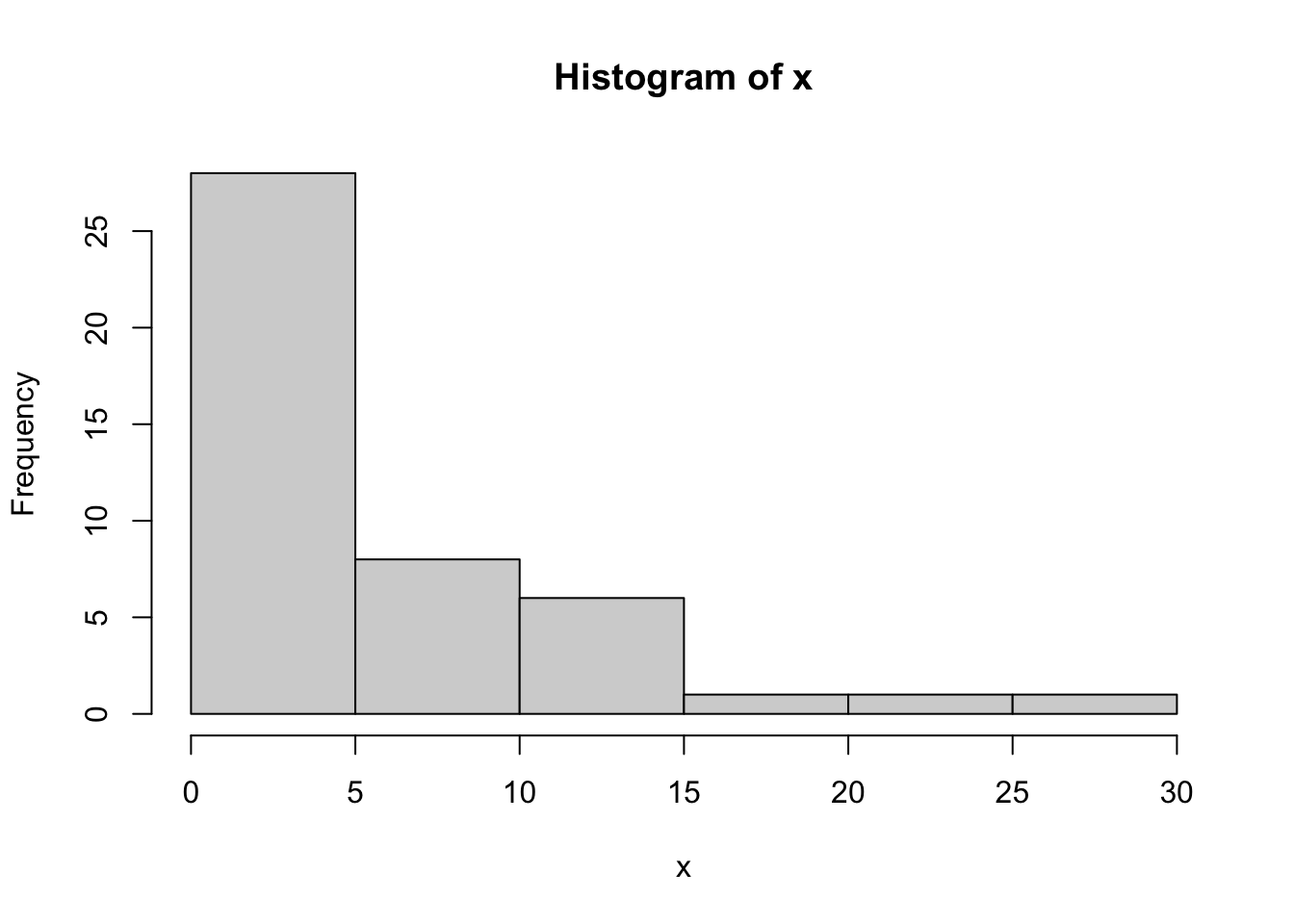
We will walk through the numerical approximations using the case where we have data from a geometric distribution as follows:
## assume that x~geom(p)x=c(4,11,2,5,1,0,11,9,0,0,1,2,17,9,6,0,0,12,3,1,3,0,0,1,27,0,2,0,24,9,4,0,0,8,13,8,6,1,4,9,12,11,2,5,3)x
To find the MLE numerically, we would first write a function to evaluate the negative log likelihood as we have done before.
nll.geom=function(p,x){-sum(log(dgeom(x,p)))}
Then use optim to numerically approximate the MLE:
out=optim(0.5,nll.geom,x=x)out
$par
[1] 0.1546875

$value
[1] 125.3257

$counts
function gradient
      28       NA

$convergence
[1] 0

$message
NULL
If we run the same optim code, but include the option hessian=TRUE, then optim will approximate the Fisher Information, and return it in the optim object, with the name of hessian.
out=optim(0.5,nll.geom,x=x,hessian=TRUE)out
$par
[1] 0.1546875

$value
[1] 125.3257

$counts
function gradient
      28       NA

$convergence
[1] 0

$message
NULL

$hessian
         [,1]
[1,] 2225.054
This hessian is the Fisher Information, so we can construct an approximate asymptotic 95% confidence interval for our MLE of the parameter \(p\) by following the above formulas:
## get the MLEp.hat=out$parp.hat
[1] 0.1546875
## get the Fisher InformationI=out$hessian## get the 95% CIp.hat-1.96*sqrt(1/I)
          [,1]
[1,] 0.1131361
p.hat+1.96*sqrt(1/I)
          [,1]
[1,] 0.1962389
So a 95% CI for the MLE of \(p\) would be (0.113,0.196).
7.3.2 Multiple Parameter Case
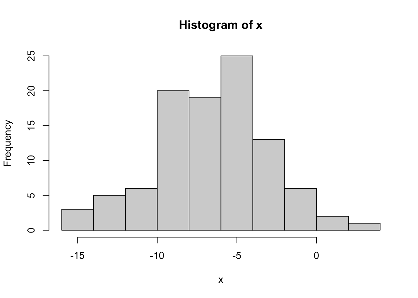
When we have two or more parameters, numeric optimization in R, as well as numeric approximation of the Fisher Information Matrix \(\mathbf{I}(\hat{\boldsymbol\theta})\) can similarly be done using optim. To illustrate this, we will consider data generated from the Normal distribution. The following code simulates normally-distributed data from a distribution with a mean of -7 and variance of 16:
The MLEs of \(\boldsymbol\theta=(\mu,\sigma^2)\) are:
theta.hat=out$partheta.hat
[1] -6.564774 12.773473
so the MLE of \(\mu\) is 5.469399 and the MLE of \(\sigma^2\) is 38.620385.
To find confidence intervals for each of these parameters, we need to find the matrix inverse of the Fisher Information \(\mathbf{I}\), and then get the square root of its diagonal elements. As these values are often called the “standard errors”, we will denote them as se in the R code:
## standard errors = sqrt(1/I.inv[p,p])I=out$hessianse=sqrt(diag(solve(I)))se
[1] 0.357400 1.805645
This gives us a vector, where the \(k\)-th entry is \(\sqrt{\mathbf{I}^{-1}(\hat{\theta}_{ML})[k,k]}\). The standard error associated with \(\mu\) is the first of these (\(se[1]\)) and the standard error associated with \(\sigma^2\) is the second of these. The order is the same as the order of the parameter estimates in out\$par. We can thus construct 95% CIs for \(\mu\)
## CI for muc(theta.hat[1]-1.96*se[1] , theta.hat[1]+1.96*se[1])
[1] -7.265278 -5.864270
and for \(\sigma^2\):
## CI for sigma^2c(theta.hat[2]-1.96*se[2] , theta.hat[2]+1.96*se[2])
This result is powerful because it allows us to use normal-based methods, like confidence intervals and hypothesis tests, even in complex models. The takeaway: MLEs are not only useful but also come with strong theoretical guarantees as sample size grows.
7.4 Summary
In this lesson we gained practical skills to analyze data using maximum likelihood estimation (MLE) and construct reliable confidence intervals. We can now calculate MLEs for parameters in distributions like Bernoulli, exponential, and normal, and use the Fisher Information to quantify uncertainty and build asymptotic confidence intervals. With R’s optim function, we can numerically estimate MLEs and intervals for complex models, such as geometric or normal distributions, even when analytical solutions are elusive.
We also learned to apply parametric and nonparametric bootstrap methods to generate confidence intervals from data, as demonstrated with t-distributed and Pareto datasets, enabling robust inference without strict distributional assumptions.
Looking ahead, the bootstrap confidence interval techniques we’ve mastered will be invaluable for tackling real-world datasets with non-standard distributions or small sample sizes, empowering you to make data-driven decisions in future statistical analyses.
Source Code
---categories: [MLEs, Asymptotic Confidence Intervals, Numerical Approximations, Bootstrap]image: /assets/415lesson7thumb.pngfile-modified:execute: freeze: true---# Asymptotic Distribution of MLE (Part I)## Overview {.unnumbered .unlisted}Let’s revisit maximum likelihood estimators (MLEs) to explore their asymptotic properties and their application in constructing confidence intervals. This lesson introduces the theoretical foundations of MLEs, including their consistency, equivariance, and asymptotic normality under regularity conditions. You will learn to derive the Fisher Information for single and multiple parameter models and use it to construct asymptotic confidence intervals. The lesson also covers numerical approximations of these intervals using R’s `optim` function. Let us dive in.::: objectiveblock<i class="bi bi-check2-circle"></i>[Objectives]{.callout-header}Upon completion of this lesson, you should be able to:1. Apply to Properties of the MLE to find an asymptotic Confidence Interval for $\theta$,2. Analytically find asymptotic confidence intervals using MLEs, and3. Use R to numerically find an asymptotic confidence interval for $\theta$ using the MLE.:::## Properties of MLEsMaximum likelihood estimation is popular because there are a number of provable properties that apply to **ANY MLE!**The following result holds for any MLE, subject to some "regularity conditions". The regularity conditions include- The underlying probability function, $f(x|\theta)$, is "smooth".- The estimator, $\hat{\theta}_{mle}$, is NOT on the edge of allowable values. For example, the MLE is not in the support.We will not show the full list of conditions nor proofs of the following properties. You can find them in the Wasserman text, chapter 9.13.::: {.callout-tip .bg-success-subtle appearance="minimal"}#### Property 1: The estimator, $\hat{\theta}_{mle}$ is consistent.This means that as the sample size $n$ approaches infinity, $\hat{\theta}_{mle}$ approaches the true $\theta$. A corollary to this is as $n$ approaches infinity, $E(\hat{\theta}_{mle})$ approaches the true $\theta$.:::::: {.callout-tip .bg-success-subtle appearance="minimal"}#### Property 2: The estimator, $\hat{\theta}_{mle}$, is equivariant.An estimator, $\hat{\theta}$, is the MLE of $\theta$, and $g(\theta)$ is an invertible function, then the MLE of $\tau=g(\theta)$ is $\hat{\tau}=g(\hat{\theta})$.This means that MLE of a function of a parameter is the function of the MLE of the parameter, as long as the function is invertible.:::::: {#exm-mle1}Let $X_i\sim N(\mu, \sigma^2)$. That is, let $X_1, X_2, \ldots, X_n$ be iid Normal random variables with mean $\mu$ and variance $\sigma^2$. We know that $\hat{\mu}=\bar{x}$ and $\hat{\sigma}^2=\frac{1}{n}\sum_{i=1}^n(x_i-\bar{x})^2$ are the MLEs of $\mu$ and $\sigma^2$, respectfully. What is the MLE of the standard deviation, $\sigma$?::: {.card .card-body .bg-light .ms-3 .mb-3 .pt-0}#### SolutionWe know $\sigma=g(\sigma^2)=\sqrt{\sigma^2}$. Therefore, based on the equivariant property, the MLE of $\sigma$ is: \begin{align*} \hat{\sigma}_{mle}=\sqrt{\hat{\sigma}^2_{mle}}=\sqrt{\frac{1}{n}\sum_{i=1}^n (x_i-\bar{x})^2}\end{align*}::::::::: {#exm-mle2}Let $X_i\sim Bin(5, p)$, for $i=1, \ldots, n$. What is the MLE of the odds ratio, $\text{OR}=\frac{p}{1-p}$?::: {.card .card-body .bg-light .ms-3 .mb-3 .pt-0}#### SolutionThe MLE of $p$ is $\hat{p}=\dfrac{\sum_{i=1}^n x_i}{5n}$.Therefore, the MLE of $\text{OR}$ is \begin{align*} \hat{\text{OR}}_{mle}=\dfrac{\hat{p}}{1-\hat{p}}=\dfrac{\dfrac{\sum_{i=1}^n x_i}{5n}}{1-\dfrac{\sum_{i=1}^n x_i}{5n}}\end{align*}::::::::: {.callout-tip .bg-success-subtle appearance="minimal"}#### Property 3: MLEs are Asymptotically Normal.For $X_i\sim f(x_i|\theta)$ $i=1, \ldots, n$, the MLE is $\hat{\theta}=\text{argmax}_{\theta}(L(\theta))$. As $n$ approaches infinity, the MLE $\hat{\theta}$ is approximately normal: $$\begin{align*} \hat{\theta}\approx N\left(\theta_{\text{true}}, \frac{1}{I(\hat{\theta}_{mle})}\right)\end{align*}$$Here "$\approx$" means "is approximately distributed as". The function $I(\theta)$ is called the "**Fisher Information**" or the "Information" function. It is defined as$$\begin{align*} I(\hat{\theta}_{mle})=-E\left(\frac{d^2}{d\theta^2}\ell(\hat{\theta})\right)\end{align*}$$:::::: {#exm-mle3}Let $X_1, \ldots, X_n$ be an i.i.d. sample from a Bernoulli distribution with parameter $p$. Find the MLE of $p$ and find $I(\hat{p})$. Then find the approximate normal distribution of $\hat{p}$.::: {.card .card-body .bg-light .ms-3 .mb-3 .pt-0}#### SolutionThe pmf is $f(x|p)=p^x(1-p)^{1-x}$. The likelihood function is:$$L(p)=\prod_{i=1}^n p^{x_i}(1-p)^{1-x_i}=p^{\sum x_i}(1-p)^{n-\sum x_i}$$The log-likelihood function is: $$\ell(p)=\sum x_i \ln(p)+(n-\sum x_i)\ln (1-p)$$The derivative of the log-likelihood function is: $$\frac{d}{dp}\ell(p)=\frac{\sum x_i}{p}-\frac{n-\sum x_i}{1-p}$$Setting the derivative equal to zero we get:::: {style="overflow-x:auto;overflow-y:hidden;"}```{=tex}\begin{align*} & 0=\frac{\sum x_i}{p}-\frac{n-\sum x_i}{1-p}, \qquad \Rightarrow 0=\frac{\sum x_i -p\sum x_i -np+p\sum x_i}{p(1-p)}\\ & 0=\sum x_i-np, \qquad \hat{p}=\frac{\sum x_i}{n}\end{align*}```:::Therefore, the MLE of $p$ is $\hat{p}=\dfrac{\sum x_i}{n}$. Next, lets find $I(p)=-E\left(\frac{d^2}{dp^2}\ell(p)\right)$.$$\frac{d^2}{dp^2}\ell(p) = -\frac{\sum x_i}{p^2}-\frac{n-\sum x_i}{(1-p)^2}$$Next, we need to find the negative expectation of the second derivative. \begin{align*} I(p)&=-E\left(\frac{d^2}{dp^2}\ell(p)\right)\\ &=-E\left(-\frac{\sum x_i}{p^2}-\frac{n-\sum x_i}{(1-p)^2}\right)\\ &=E\left(\frac{\sum x_i}{p^2}+\frac{n-\sum x_i}{(1-p)^2}\right)\\ &=\frac{\sum E(x_i)}{p^2}+\frac{n-\sum E(x_i)}{(1-p)^2}\end{align*}For a Bernoulli random variable $E(X)=p$. Therefore, \begin{align*} I(p)&=\frac{\sum E(x_i)}{p^2}+\frac{n-\sum E(x_i)}{(1-p)^2}\\ &=\frac{np}{p^2}+\frac{n-np}{(1-p)^2}\\ &=\frac{np(1-p)^2+np^2-np^3}{p^2(1-p)^2}\\ & =\frac{np((1-p)^2+p(1-p))}{p^2(1-p)^2}\\ &=\frac{np(1-p)(1-p+p)}{p^2(1-p)^2}\\ &=\frac{n}{p(1-p)}\end{align*}If $I(p)=\frac{n}{p(1-p)}$, then $I(\hat{p})=\dfrac{n}{\hat{p}(1-\hat{p})}=\dfrac{n}{\dfrac{\sum x_i}{n}\left(1-\dfrac{\sum x_i}{n}\right)}=\dfrac{n}{\bar{x}(1-\bar{x})}$.Putting this all together, we have $\hat{p}\approx N\left(p_{true}, \dfrac{1}{I(\hat{p})}\right)$. Which is equivalent to $\hat{p}\approx N\left(p_{true}, \dfrac{\bar{x}(1-\bar{x})}{n}\right)$.::::::Now that we have determined an asymptotic distribution of MLEs (under certain conditions), we can use this information (with large sample size) to construct interval estimates for our unknown parameter, $\theta$.## Asymptotic Confidence Intervals### Single Parmater CaseIn this section, we put together the Properties discussed in the previous section to construct an asymptotic confidence interval for the unknown parameter, $\theta$, using the MLE.The normal approximation to the distribution of any MLE gives us an easy way to find an asymptotic confidence interval for the unknown parameter.::: {.callout-tip .bg-success-subtle appearance="minimal"}#### Property 4: Approximate Confidence IntervalLet $X_i$ follow a distribution with probability distribution $f(x_i|\theta)$. Let $\hat{\theta}$ be the MLE of $\theta$. We have $I(\theta)=-E\left(\frac{d^2}{d\theta^2} \ell(\theta)\right)$. Then an asymptotic 95% confidence interval for $\theta$ is \begin{align*} \hat{\theta}\pm 1.96 \sqrt{\frac{1}{I(\hat{\theta})}}\end{align*}:::::: {#exm-mle4}Continuing the previous example, we know $\hat{p}=\bar{x}$, $I(\hat{p})=\frac{n}{\bar{x}(1-\bar{x})}$, and $\hat{p}\approx N\left(p_{true}, \frac{\bar{x}(1-\bar{x})}{n}\right)$. Find a 95% asymptotic confidence interval for $p$.::: {.card .card-body .bg-light .ms-3 .mb-3 .pt-0}#### SolutionAn approximate 95% confidence interval for $p$ is:```{=tex}\begin{align*} \bar{x}\pm 1.96 \sqrt{\frac{\bar{x}(1-\bar{x})}{n}}\end{align*}```::::::::: {#exm-mle4b}Suppose we have the following 10 observations from a Bernoulli distribution with parameter $p$. Calculate a 95% asymptotic confidence interval for $p$.|||||||-----|-----|-----|-----|-----|| 1 | 1 | 0 | 1 | 0 || 0 | 0 | 1 | 1 | 1 |: {.w-auto .table-sm .mx-auto}::: {.card .card-body .bg-light .ms-3 .mb-3 .pt-0}#### SolutionContinuing the previous example, we know $\hat{p}=\bar{x}$, $I(\hat{p})=\dfrac{n}{\bar{x}(1-\bar{x})}$, and $\hat{p}\approx N\left(p_{true}, \dfrac{\bar{x}(1-\bar{x})}{n}\right)$.We can calculate $\bar{x}=0.6$ and know $n=10$. Therefore,An approximate 95% confidence interval for $p$ is:```{=tex}\begin{align*} \bar{x}\pm 1.96 \sqrt{\frac{\bar{x}(1-\bar{x})}{n}}=0.6\pm \sqrt{\frac{0.6(1-0.6)}{10}}=0.6\pm 0.3036=(0.2964, 0.9036)\end{align*}```::: {.callout-caution appearance="minimal"}**Note!** \The sample size is not large in this example but it is chosen it for practice purposes.:::::::::::: {#exm-mle5}Let $X_1, X_2, \ldots, X_n$ be a random sample from $\text{Exp}(\theta)$. Find a 95% asymptotic CI for $\theta$, using the MLE of $\theta$.::: {.card .card-body .bg-light .ms-3 .mb-3 .pt-0}#### SolutionThe PMF is $f(x_i|\theta)=\frac{1}{\theta}e^{-\frac{x_i}{\theta}}$ and $E(X_i)=\theta$.**Step 1**: Find the likelihood function.$$\begin{align*} L(\theta)=\prod_{i=1}^n \frac{1}{\theta}e^{-\frac{x_i}{\theta}}=\theta^{-n}e^{-\frac{\sum x_i}{\theta}}\end{align*}$$**Step 2**: Find the log-likelihood function.$$\begin{align*} \ell(\theta)=-n\log \theta -\frac{\sum x_i}{\theta}\end{align*}$$**Step 3**: Find the derivative of the log-likelihood function with respect to $\theta$.$$\begin{align*} \frac{d}{d\theta}=-\frac{n}{\theta}+\frac{\sum x_i}{\theta^2}\end{align*}$$**Step 4**: Set the derivative equal to 0 and solve for $\theta$.$$\begin{align*} & 0=\frac{-n\theta+\sum x_i}{\theta^2}, \qquad \Rightarrow 0=-n\theta+\sum x_i\\ & \Rightarrow \hat{\theta}=\frac{\sum x_i}{n}\end{align*}$$**Step 5**: Find $I(\hat{\theta})=-E\left(\frac{d^2}{d\theta^2}\ell(\hat{\theta})\right)$.$$\begin{align*} \frac{d^2}{d\theta^2}\ell(\theta)&=\frac{n}{\theta^2}-\frac{2\sum x_i}{\theta^3}\\ &=\frac{n\theta -2\sum x_i}{\theta^3}\\ I(\hat{\theta})&=-E\left[\frac{n\theta -2\sum x_i}{\theta^3}\right]\\&=-\frac{n\hat{\theta} -2\sum x_i}{\hat{\theta}^3}\\ &=-\frac{n\hat{\theta}-2n\hat{\theta}}{\hat{\theta}^3}=\frac{n}{\bar{x}^2}=\frac{n}{\hat{\theta}^2}=\frac{n^3}{(\sum x_i)^2}\end{align*}$$Therefore, a 95% asymptotic confidence interval for $\theta$ is: $$\hat{\theta}\pm 1.96\sqrt{\frac{1}{I(\hat{\theta})}}=\bar{x}\pm 1.96 \sqrt{\frac{n^3}{\bar{x}^2}}$$::::::### Multiple Parmater CaseIn the multivariate case, where there are two or more parameters to be estimated, $\boldsymbol\theta=(\theta_1,\theta_2,\ldots,\theta_p)$ is the vector of $p$ parameters to be estimated and the asymptotic distribution is as follows. as $n\rightarrow \infty$, $$ \hat{\boldsymbol\theta}_{ML}\sim N\left(\boldsymbol\theta_{\text{true}},\mathbf{I}^{-1}(\hat{\boldsymbol\theta}_{ML})\right)$$ where $\mathbf{I}(\boldsymbol\theta)$ is the "Fisher Information Matrix", defined by $$\mathbf{I}(\boldsymbol\theta) = \left[\begin{array}{cccc}-E_x\left[\frac{\partial^2}{\partial \theta_1^2}\ell(\theta)\right] & -E_x\left[\frac{\partial^2}{\partial \theta_1\partial\theta_2}\ell(\theta)\right] & \cdots & -E_x\left[\frac{\partial^2}{\partial \theta_1\partial\theta_p}\ell(\theta)\right]\\-E_x\left[\frac{\partial^2}{\partial \theta_2\partial\theta_1}\ell(\theta)\right] & -E_x\left[\frac{\partial^2}{\partial\theta_2^2}\ell(\theta)\right] & \cdots & -E_x\left[\frac{\partial^2}{\partial \theta_2\partial\theta_p}\ell(\theta)\right]\\\vdots & \vdots & & \vdots \\-E_x\left[\frac{\partial^2}{\partial \theta_p\partial\theta_1}\ell(\theta)\right] & -E_x\left[\frac{\partial^2}{\partial \theta_p\partial\theta_2}\ell(\theta)\right] & \cdots & -E_x\left[\frac{\partial^2}{\partial \theta_p^2}\ell(\theta)\right] \end{array}\right]$$ where again $\ell(\theta)=log(L(\theta))$ and the expectation is taken over all $x_1,x_2,\ldots,x_n$.### Summary: The Asymptotic 95% Confidence IntervalFor any MLE, the asymptotic Gaussian distribution approximation can be used to construct a confidence interval. Let $x_i\sim f_X(x|\theta)$, $i=1,2,\ldots,n$ be $n$ independent and identically distributed random variables from a distribution with only a single parameter $\theta$, and let $\hat{\theta}=\text{argmax}(L(\theta))$ be the MLE of the unknown parameter $\theta$. Then from the asymptotic approximate Gaussian distribution of any MLE, an approximate asymptotic 95% confidence interval for $\theta$ is $$\hat{\theta}\pm 1.96\sqrt{1/I(\hat{\theta}_{ML})}$$Similarly, for a multiparameter model, an approximate asymptotic 95% confidence interval for the $k$-the parameter $\theta_k$ is $$\hat{\theta_k}\pm 1.96\sqrt{\mathbf{I}^{-1}(\hat{\theta}_{ML})[k,k]}$$ where $\sqrt{\mathbf{I}^{-1}(\hat{\theta}_{ML})[k,k]}$ is the square root of the $k$-th diagonal entry of $\mathbf{I}^{-1}(\hat{\theta}_{ML})$ where $\mathbf{I}^{-1}$ is the matrix inverse of $\mathbf{I}$.## Numerical Approximations for CIsFor some relatively simple cases, we can analytically construct 95% confidence intervals for MLEs. This requires being able to analytically find the MLE (by taking the first derivative of the log-likelihood function and setting equal to zero), and then also analytically find the Fisher Information (by taking two derivatives of the log-likelihood function and then taking the expectation over $x_1,x_2,\ldots,x_n$). As we have seen, there are many cases, even for simple statistical distributions, where it is impossible to analytically solve for the MLE. In these cases we numerically approximated this MLE by using `optim` in R. Just like we can approximate the MLE using `optim`, we can also approximate the Fisher Information $I(\hat{\theta})$ (in the single-parameter case) or $\mathbf{I}(\hat{\boldsymbol\theta})$ (in the multiparameter case) using `optim`. We do this in `optim` by including one additional input in our call to `optim`.### Single Parameter CaseWe will walk through the numerical approximations using the case where we have data from a geometric distribution as follows:::: {#fig-histoofx}```{r message=FALSE, warning=FALSE, error=FALSE, out.width="70%"}#| fig-alt: Histogram of geometric distribution#| eval: true#| echo: true#| lightbox: true## assume that x~geom(p)x=c(4,11,2,5,1,0,11,9,0,0,1,2,17,9,6,0,0,12,3,1,3,0,0,1,27,0,2,0,24,9,4,0,0,8,13,8,6,1,4,9,12,11,2,5,3)xhist(x)```:::To find the MLE numerically, we would first write a function to evaluate the negative log likelihood as we have done before.```{r}nll.geom=function(p,x){-sum(log(dgeom(x,p)))}```Then use `optim` to numerically approximate the MLE:```{r}out=optim(0.5,nll.geom,x=x)out```If we run the same `optim` code, but include the option `hessian=TRUE`, then `optim` will approximate the Fisher Information, and return it in the `optim` object, with the name of `hessian`.```{r}out=optim(0.5,nll.geom,x=x,hessian=TRUE)out```This `hessian` is the Fisher Information, so we can construct an approximate asymptotic 95% confidence interval for our MLE of the parameter $p$ by following the above formulas:```{r}## get the MLEp.hat=out$parp.hat## get the Fisher InformationI=out$hessian## get the 95% CIp.hat-1.96*sqrt(1/I)p.hat+1.96*sqrt(1/I)```So a 95% CI for the MLE of $p$ would be (0.113,0.196).### Multiple Parameter CaseWhen we have two or more parameters, numeric optimization in R, as well as numeric approximation of the Fisher Information Matrix $\mathbf{I}(\hat{\boldsymbol\theta})$ can similarly be done using `optim`. To illustrate this, we will consider data generated from the Normal distribution. The following code simulates normally-distributed data from a distribution with a mean of -7 and variance of 16:::: {#fig-histoofnormaldistr}```{r message=FALSE, warning=FALSE, error=FALSE, out.width="70%"}#| fig-alt: Histogram of normal distribution#| eval: true#| echo: true#| lightbox: trueset.seed(1)x=rnorm(100,mean=-7,sd=sqrt(16))xhist(x)```:::To find the MLE, we first write a function to evaluate the negative log likelihood:```{r}nll.norm=function(theta,x){ mn=theta[1] vr=theta[2]-sum(log(dnorm(x,mean=mn,sd=sqrt(vr))))}```Then run `optim` to find the MLE. We include the `hessian=TRUE` option, to tell `optim` to approximate the Fisher Information Matrix.```{r}out=optim(c(-11,1),nll.norm,x=x,hessian=TRUE)out```The MLEs of $\boldsymbol\theta=(\mu,\sigma^2)$ are:```{r}theta.hat=out$partheta.hat```so the MLE of $\mu$ is 5.469399 and the MLE of $\sigma^2$ is 38.620385.To find confidence intervals for each of these parameters, we need to find the matrix inverse of the Fisher Information $\mathbf{I}$, and then get the square root of its diagonal elements. As these values are often called the "standard errors", we will denote them as `se` in the R code:```{r}## standard errors = sqrt(1/I.inv[p,p])I=out$hessianse=sqrt(diag(solve(I)))se```This gives us a vector, where the $k$-th entry is $\sqrt{\mathbf{I}^{-1}(\hat{\theta}_{ML})[k,k]}$. The standard error associated with $\mu$ is the first of these ($se[1]$) and the standard error associated with $\sigma^2$ is the second of these. The order is the same as the order of the parameter estimates in `out\$par`. We can thus construct 95% CIs for $\mu$```{r}## CI for muc(theta.hat[1]-1.96*se[1] , theta.hat[1]+1.96*se[1])```and for $\sigma^2$:```{r}## CI for sigma^2c(theta.hat[2]-1.96*se[2] , theta.hat[2]+1.96*se[2])```and also **asymptotically normal**:$$\sqrt{n}(\hat{\theta}_{\text{MLE}} - \theta) \xrightarrow{d} \mathcal{N}\left(0, \frac{1}{I(\theta)}\right)$$Here, $I(\theta)$ is the **Fisher Information**, which quantifies how much information the data gives us about the parameter. It is defined as:$$I(\theta) = \mathbb{E} \left[ \left( \frac{\partial}{\partial \theta} \log f(X \mid \theta) \right)^2 \right]$$This result is powerful because it allows us to use normal-based methods, like confidence intervals and hypothesis tests, even in complex models. The takeaway: MLEs are not only useful but also come with strong theoretical guarantees as sample size grows.## SummaryIn this lesson we gained practical skills to analyze data using maximum likelihood estimation (MLE) and construct reliable confidence intervals. We can now calculate MLEs for parameters in distributions like Bernoulli, exponential, and normal, and use the Fisher Information to quantify uncertainty and build asymptotic confidence intervals. With R’s `optim` function, we can numerically estimate MLEs and intervals for complex models, such as geometric or normal distributions, even when analytical solutions are elusive.