y=c(-0.71,-1.30,-0.13,-2.03, 1.62, 2.38, 0.48, 0.51,-0.69,
    -2.32,-2.02,1.23,-0.25,0.76,0.65,-0.08,-1.20,0.99,
    2.58,0.73,-0.09,-0.03,0.56,-1.44,0.13)
hist(y)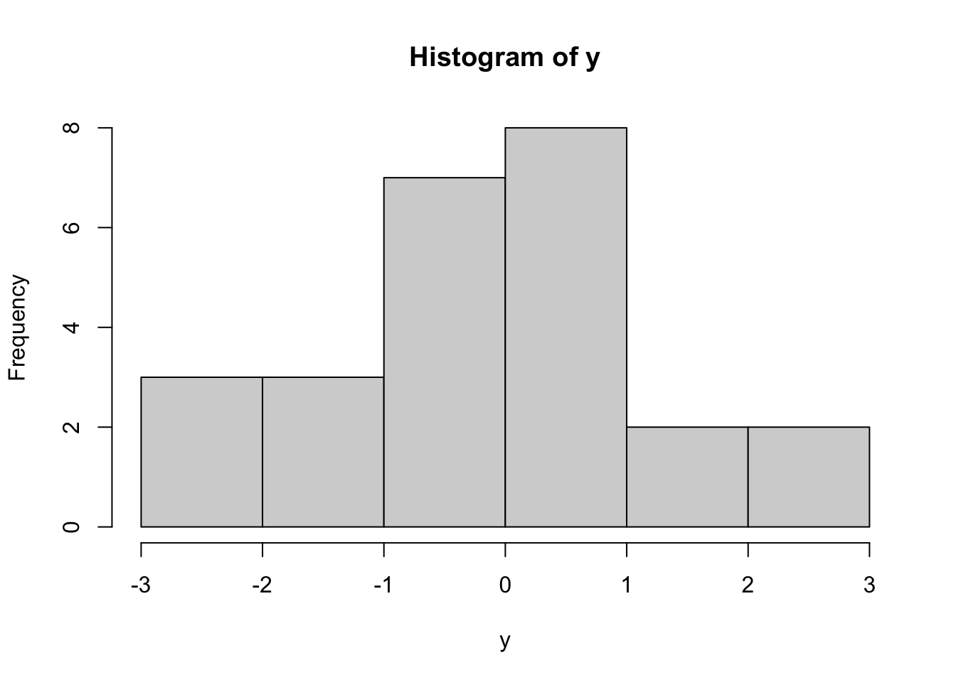
This lesson introduces the bootstrap method—both parametric and nonparametric—for estimating confidence intervals when analytical solutions are infeasible. Additionally, you will explore the Delta method and bootstrap approaches for inference on transformations of parameters. Through examples involving Bernoulli, exponential, normal, geometric, t, and Pareto distributions, you will gain practical skills in applying these techniques, preparing you for advanced statistical inference.
Objectives
Upon completion of this lesson, you should be able to:
The confidence intervals constructed above rely on us knowing an approximate distribution for our estimate \(\hat{\theta}\) of the parameter \(\theta\). We have relied on the asymptotic Normal (Gaussian) approximation for any MLEs above, but there are other ways to find an approximate distribution of an estimate \(\hat{\theta}\).
One incredibly common approach for finding an approximate sampling distribution of an estimator is the bootstrap. A bootstrap is an approach that relies on random samples from an approximate distribution, instead of on an actual defined distribution. The benefit of relying on samples is that we do NOT need to actually know the distribution we are sampling from, we just need to be able to sample from this distribution!
The goal of any bootstrap is to construct a method for sampling from the distribution of the estimator. Bootstraps typically do this by (1) approximating the distribution of the data, and then (2) simulating many data sets from that distribution. Each of those simulated data sets is approximately distributed the same as the true data, and each simulated data set could be used to find an estimate of the parameter of interest. Doing so results in (3) many parameter estimates, each a realization from the approximate sampling distribution of the estimator. We don’t know the distribution of these estimates, but we have many samples from this distribution, so we can (4) approximate confidence intervals or other quantities by looking at sample-based approximations.
In other words, the bootstrap steps are:
(1)-(2): Simulate \(m\) data sets of \(n\) from the approximate distribution of the data.
(3): Calculate \(\hat{\theta}_i\) from each data set, \(i=1, \ldots, m\).
(4): Using the parameter estimates from step (3), obtain an approximate confidence interval.
In the next section, we demonstrate an example.
To illustrate this, consider the following data from a t-distribution. We will simulate data here:
y=c(-0.71,-1.30,-0.13,-2.03, 1.62, 2.38, 0.48, 0.51,-0.69,
-2.32,-2.02,1.23,-0.25,0.76,0.65,-0.08,-1.20,0.99,
2.58,0.73,-0.09,-0.03,0.56,-1.44,0.13)
hist(y)
These data are independent of each other and come from \(y_i \sim t(4)\), a t-distribution with degrees of freedom parameter equal to 4. If we did not know the true value of the degrees of freedom (\(\text{df}\)) parameter, we could first try to find the maximum likelihood estimate directly. However, the pdf of a t-distribution does not result in an analytically solvable MLE. We can find it from the data using numerical maximum likelihood estimation. Numerical inference in R could be done by writing a negative log-likelihood function, and then optimizing using optim.
## negative log-likelihood function
nll.t=function(df,y){
    -sum(dt(y,df=df,log=TRUE))
}
## run optim
out=optim(1,fn=nll.t,y=y,hessian=TRUE)
## get mle
df.hat=out$par
df.hat
[1] 6.63125We see that our MLE for \(\text{df}\) is \(\hat{\text{df}}=6.63125\).
We could then construct a confidence interval using the asymptotic Normal approximation for MLEs, as follows:
## Get Fisher Information
I=out$hessian
## Get CI
c(df.hat-1.96*sqrt(1/I),df.hat+1.96*sqrt(1/I))
[1] -6.6074 19.8699Note that this confidence interval is quite wide, and in fact includes negative values, which are impossible for the degrees of freedom parameter in a t-distribution!
This confidence interval relies on a Normal distribution approximation which is known to be an accurate approximation as the sample size \(n\) goes to infinity. However, for any fixed sample size (\(n=25\) here), we don’t know how good the approximation is. As a normal distribution has as its support the whole real line, negative values are reasonable in that approximate distribution. Since the \(\text{df}\) parameter must be positive, we know that this approximate distribution may not be a great one for our current situation.
In the next section, we present another way to construct an approximate confidence interval using bootstrap samples. We will discuss the parametric bootstrap and the nonparametric bootstrap.
The first bootstrap we will learn is the parametric bootstrap. In any bootstrap method, we need a way to simulate data from an approximation to the distribution that gave rise to the data.
In the parametric bootstrap, we do this by first estimating the parameters in the data model, then using those estimated parameters as parameters in the data model to simulate data.
Let \(x_i\sim f_X(x_i|\theta)\), \(i=1, \ldots, n\), be independent data points that we assume come from the distribution \(f_X(x|\theta)\) which relies on an unknown parameter \(\theta\).
The parametric bootstrap algorithm is as follows:
This estimation could be done using analytic MLE, numeric MLE, or even some other approach, like method of moments.
Each of the data set are the same size \(n\) as the original data, and each from \(x_i^{(m)}\sim f_X(x|\hat{\theta})\).
This results in \(M\) different parameter estimates: \(\{\hat{\theta}^{(1)},\hat{\theta}^{(2)},\ldots,\hat{\theta}^{(M)}\}\), each from a different simulated data set \[ \{x_1^{(1)},x_2^{(1)},\ldots,x_n^{(1)}\} \rightarrow \hat{\theta}^{(1)}\] \[ \{x_1^{(2)},x_2^{(2)},\ldots,x_n^{(2)}\} \rightarrow \hat{\theta}^{(2)}\] \[ \vdots \] \[ \{x_1^{(M)},x_2^{(M)},\ldots,x_n^{(M)}\} \rightarrow \hat{\theta}^{(M)} \] This set of \(M\) parameter estimates are approximately distributed as samples from the distribution of our parameter estimate \(\hat{\theta}\), with the approximation coming from the fact that we simulated data from \(f_X(x|\hat{\theta})\) - the generating distribution of the data assuming that the true parameter is our estimate \(\hat{\theta}\), instead of from the true generating distribution \(f_X(x|\theta)\).
For example, if we are interested in a 95% confidence interval on \(\theta\), we could approximate it with a 95% probability interval of this sampling distribution, by finding the .025 and .975 quantile of the samples \(\{\hat{\theta}^{(1)},\hat{\theta}^{(2)},\ldots,\hat{\theta}^{(M)}\}\). \[ 95\% \text{ CI on } \theta \approx \left(\hat{q}_{.025}\left\{\hat{\theta}^{(1)},\hat{\theta}^{(2)},\ldots,\hat{\theta}^{(M)}\right\}\ ,\ \hat{q}_{.975}\left\{\{\hat{\theta}^{(1)},\hat{\theta}^{(2)},\ldots,\hat{\theta}^{(M)}\right\}\right)\] To approximate a .025 and .975 quantile well, we will need a large number \(M\) of bootstrap samples.
To illustrate this approach, we will construct a bootstrap 95% confidence interval on \(df\) from our t-distributed data example. For clarity, we will re-introduce the data and model. The data are as follows:
x=c(-0.71,-1.30,-0.13,-2.03, 1.62, 2.38, 0.48, 0.51,-0.69,
    -2.32,-2.02,1.23,-0.25,0.76,0.65,-0.08,-1.20,0.99,
    2.58,0.73,-0.09,-0.03,0.56,-1.44,0.13)
and we assume that \(x_i\sim t(\text{df})\), where \(\text{df}\) is an unknown parameter to be estimated, \(\theta\).
Following the 4 steps above:
Estimate \(\hat{\theta}\)
Using the data \(\{x_1,x_2,\ldots,x_n\}\), we estimate the parameter \(\hat{\theta}\) using numerical maximum likelihood.
## negative log-likelihood function
nll.t=function(df,y){
   -sum(dt(y,df=df,log=TRUE))
}
## run optim
out=optim(1,fn=nll.t,y=y,hessian=TRUE)
## get mle
df.hat=out$par
df.hat
[1] 6.63125The estimate of \(\theta\) is \(\hat{\theta}=6.63125\).
Simulate Bootstrap Samples
We now simulate \(M=1000\) independent data sets, each of the same size \(n=25\) as the original data, and each from \(x_i^{(m)}\sim f_X(x|\hat{\theta})\), where \(\hat{\theta}=6.63125\).
## find the size of the original data set
n=length(x)
## choose the number of bootstrap samples
M=1000
## make a list to hold the simulated data sets
sim.data=list()
## start a "for" loop, going from 1 to M=1000
for(m in 1:M){
  ## simulate the m-th data set from x[i]~dt(df.hat)
  ## note that the size "n" is the same as the size of the    original data
  sim.data[[m]]=rt(n,df=df.hat)
}
Estimate \(\{\theta^{(m)}\}\) using Bootstrap Data
Now use each of these \(M\) data sets to obtain an estimate of \(\theta\), using the same method used in step 1.
## make a vector to store the values of theta.hat
theta.hat.vals=rep(NA,M)
## start a "for" loop, going from 1 to M=1000
for(m in 1:M){
  ## estimate theta using the m-th data set
  suppressWarnings({out=optim(1,nll.t,y=sim.data[[m]])})
  ## save the MLE
  theta.hat.vals[m]=out$par
}
This gives us a vector of \(M\) estimates of \(\theta\), each resulting from finding the MLE of a simulated data set. These are called “bootstrap samples” of \(\hat{\theta}\).
To visualize them, here is a histogram:
hist(theta.hat.vals,main="Bootstrap samples",xlab="theta.hat",ylab="")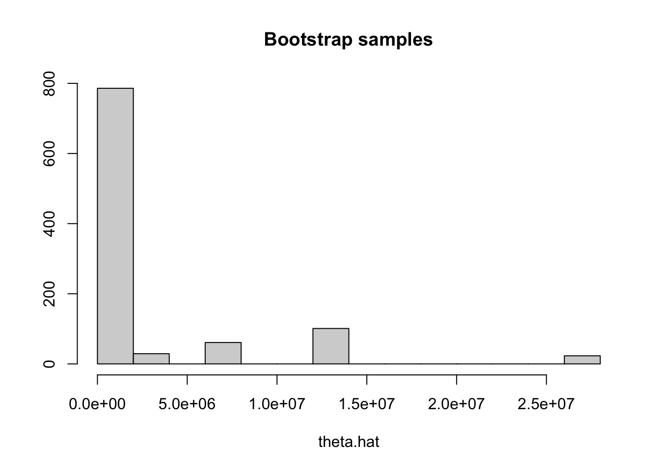
Inference on \(\hat{\theta}\)
We can now construct a 95% confidence interval from this bootstrap sample by finding its empirical .025 and .975 quantiles. This can be done using the quantile command in R:
## 95% CI
quantile(theta.hat.vals,c(.025,.975))
2.5% 97.5%
2.612500e+00 1.342177e+07 Therefore, the approximate 95% parametric bootstrap confidence interval for \(\theta=\text{df}\) is \((2.5789, 2.68\times10^7)\). While it does not contain negative values as our previous confidence interval, it is a very wide interval!
Let’s consider another bootstrap method.
The parametric bootstrap introduced above simulated new data sets from (approximately) the same distribution as our observed data by using the assumed model ( a t-distribution in the above example) and the parameters estimated from the observed data (the MLE of \(\text{df}\) in the above example).
An alternative approach to the bootstrap is to simulate new data sets directly from the observed data by resampling. This approach is called the nonparametric bootstrap.
The reasoning behind the nonparametric bootstrap is as follows. If we have observed data \(x_i \sim f_X(x)\) that are independent and identically distributed, then the best information about the distribution \(f_X\) that we have is actually the data themselves. We could approximate a new draw from \(f_X\) by just drawing, at random, one of the observed values \(x_1,x_2,\ldots,x_n\). this is called “sampling from the empirical distribution of the data”.
The empirical distribution of a set of data \(x_1,x_2,\ldots,x_n\) is a discrete distribution, with support equal to the unique values in the data \(x_1,x_2,\ldots,x_n\) and pmf defined by \[P(X=x) = \begin{cases} 1/n &,\text{ if }x=x_i \text{ for some }i\in\{1,2,\ldots,n\} \\ 0 & \text{ otherwise} \end{cases}\]
Therefore, the empirical distribution puts equal weight on each of the observed values in the dataset.
We now construct a 95% confidence interval on the \(\text{df}\) parameter of our t-distributed data using a nonparametric bootstrap.
Similar to the parametric data example, we will re-state the model and data. The data are as follows:
x=c(-0.71,-1.30,-0.13,-2.03, 1.62, 2.38, 0.48, 0.51,-0.69,
    -2.32,-2.02,1.23,-0.25,0.76,0.65,-0.08,-1.20,0.99,
    2.58,0.73,-0.09,-0.03,0.56,-1.44,0.13)
and we assume that \(x_i\sim t(\text{df})\), where \(\text{df}\) is an unknown parameter to be estimated, \(\theta\).
Following the 4 steps above:
Estimate \(\hat{\theta}\)
Using the data \(\{x_1,x_2,\ldots,x_n\}\), we estimate the parameter \(\hat{\theta}\) using numerical maximum likelihood.
## negative log-likelihood function
nll.t=function(df,y){
 -sum(dt(y,df=df,log=TRUE))
}
## run optim
out=optim(1,fn=nll.t,y=y,hessian=TRUE)
## get mle
df.hat=out$par
df.hat
[1] 6.63125Again, our estimate for \(\theta\) is \(\hat{\theta}=6.63125\).
Simulate Bootstrap Samples
We now simulate \(M=1000\) independent data sets, each of the same size \(n\) as the original data, and each from the empirical distribution. We can do this by using the sample command in R:
## find the size of the original data set
n=length(x)
## choose the number of bootstrap samples
M=1000
## make a list to hold the simulated data sets
sim.data=list()
## start a "for" loop, going from 1 to M=1000
for(m in 1:M){
  ## simulate the m-th data set from the empirical distribution
  ## note that the size "n" is the same as the size of the original data
  sim.data[[m]]=sample(x,size=n,replace=TRUE)
}
Estimate \(\{\theta^{(m)}\}\) using Bootstrap Data
Now use each of these \(M\) data sets to obtain an estimate of \(\theta\), using the same method used in step 1.
## make a vector to store the values of theta.hat
theta.hat.vals=rep(NA,M)
## start a "for" loop, going from 1 to M=1000
for(m in 1:M){
  ## estimate theta using the m-th data set
  suppressWarnings({out=optim(1,nll.t,y=sim.data[[m]])})
  ## save the MLE
  theta.hat.vals[m]=out$par
}
This gives us a vector of \(M\) estimates of \(\theta\), each resulting from finding the MLE of a simulated data set. These are called “bootstrap samples” of \(\hat{\theta}\).
To visualize them, here is a histogram
hist(theta.hat.vals,main="Bootstrap samples (nonparametric bootstrap)",xlab="theta.hat",ylab="")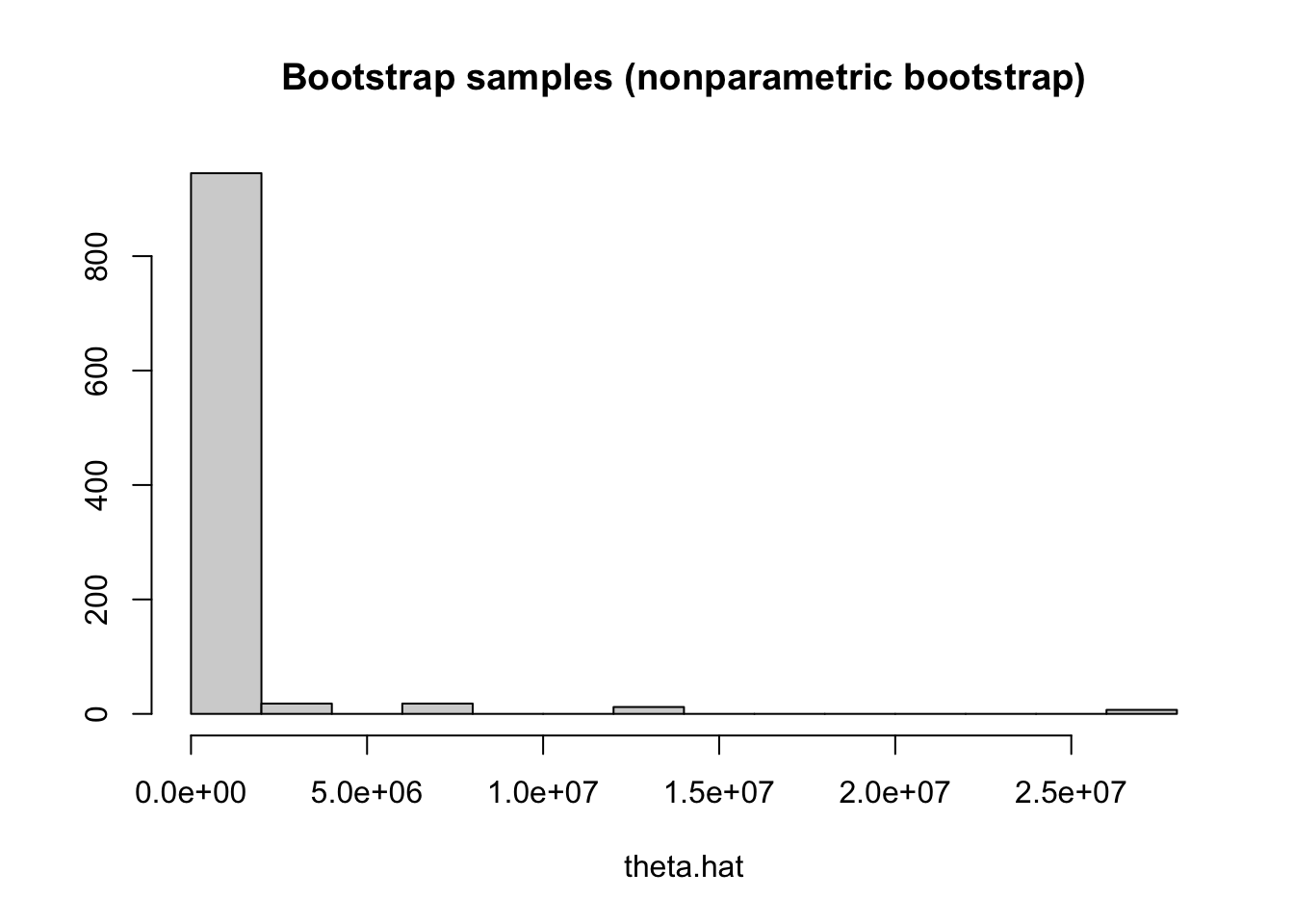
Inference on \(\hat{\theta}\)
We can now construct a 95% confidence interval from this nonparametric bootstrap sample by finding its empirical .025 and .975 quantiles. This can be done using the quantile command in R:
## 95% CI
quantile(theta.hat.vals,c(.025,.975))
2.5% 97.5%
3.339766e+00 6.710887e+06 Therefore, the approximate 95% nonparametric bootstrap confidence interval for \(\text{df}=\theta\) is \((3.2688, 6.8787\times 10^6)\). It is not as wide as the parametric interval but it is still very wide!
To make it easier to apply bootstrap methods, here is a set of template code, with some comments.
In the code below, you will need to make the following changes: a. change the data line to read in your data b. change the nll function to be the correct negative log likelihood function for your data and model.c. within the for loop, change the rexp code to be code to simulate from your model, with parameters being the MLEs from step (1). d. within the for loop, make the opti line be identical to your optim line in step (1), except that the data for the optim call within the for loop should be x=sim.data[[m]].
## read in data
x=c(1,2,3)

## (1) find the MLE using `optim`
nll=function(theta,x){
  ## code for negative log likelihood goes here!
}
out=optim(...,nll,x=x)
theta.hat=out$par
## Prepare for bootstrap
M=1000
n=length(x)
sim.data=list()
theta.hat.vals=rep(NA,n)

## "for" loop for bootstrap
for(m in 1:M){
  ## (2) simulate new data
  ## CHANGE the rexp(...) to be code to simulate data from your model
  sim.data[[m]]=rexp(n,theta.hat)
  ## (3) find the MLE using this simulated data
  ## this optim code should be the same as above, except for the data set
  out.sim=optim(...,nll,x=sim.data[[m]])
  theta.hat.vals[m]=out.sim$par
}

## (4) find a 95% CI using the bootstrap samples
quantile(theta.hat.vals,c(.025,.975))
In the code below, you will need to make the following changes: a. change the data line to read in your data b. change the nll function to be the correct negative log likelihood function for your data and model.c. within the for loop, make the optim line be identical to your optim line in step (1), except that the data for the optim call within the for loop should be x=sim.data[[m]].
## read in data
x=c(1,2,3)

## (1) find the MLE using `optim`
nll=function(theta,x){
  ## code for negative log likelihood goes here!
}
out=optim(...,nll,x=x)
theta.hat=out$par
## Prepare for bootstrap
M=1000
n=length(x)
sim.data=list()
theta.hat.vals=rep(NA,n)

## "for" loop for bootstrap
for(m in 1:M){
  ## (2) simulate new data
  sim.data[[m]]=sample(x,size=n,replace=TRUE)
  ## (3) find the MLE using this simulated data
  ## this optim code should be the same as above, except for the data set
  out.sim=optim(...,nll,x=sim.data[[m]])
  theta.hat.vals[m]=out.sim$par
}

## (4) find a 95% CI using the bootstrap samples
quantile(theta.hat.vals,c(.025,.975))Example 8.1 Consider the following data, which we assume come from a Pareto distribution
## load the library needed for "dpareto"
library(EnvStats)
## read in data
x=c(5.92, 10.87,  6.50, 14.62, 20.49,  5.12,  7.28, 15.24,
   7.47,  6.78, 24.07, 6.76,  8.81,  7.65,  5.28, 15.80,
   5.76,  5.11,  6.10, 23.44, 15.04,  9.02,  8.34, 66.05,
   8.52,  9.26,  7.40,  7.85,  5.93,  5.41, 26.00, 16.00,
   8.99, 11.06,  5.06,  6.92, 10.17,  5.65,  6.06,  5.70)
hist(x)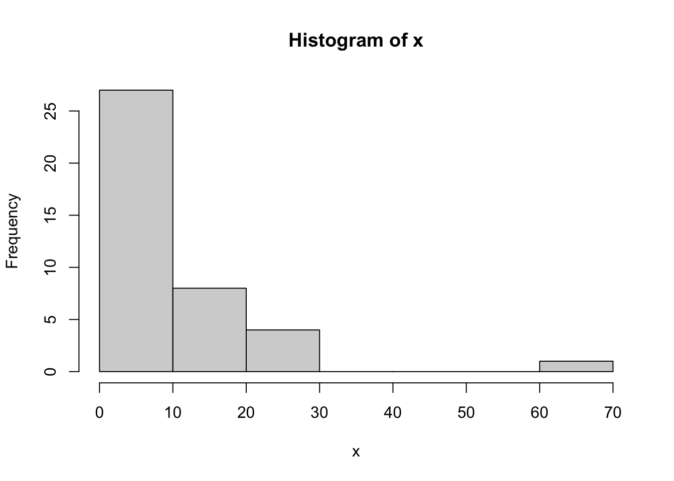
Let \(x_i \sim \text{Pareto}(L,a)\) for \(1, \ldots, n\), where \(a\) is a “shape” parameter and \(L\) is a “location” parameter which is the minimum possible value of \(x_i\). That is, the support of this distribution is \(x_i \in (L,\infty)\).
If we assume that we do not know the true values of the parameters, then we can estimate both parameters using numeric maximum likelihood estimation, and then find 95% confidence intervals for both parameters using a bootstrap.
We will use a non-parametric bootstrap below and will modify the template code from the previous section. The major change we make to it is to allow for two parameters, instead of just one.
## (1) find the MLE using `optim`
nll.pareto=function(theta,x){
  ## code for negative log likelihood goes here!
  L=theta[1]
  a=theta[2]
  -sum(log(dpareto(x,location=L,shape=a)))
}
out=optim(c(1,1),nll.pareto,x=x)
theta.hat=out$par
L.hat=theta.hat[1]
a.hat=theta.hat[2]
## Prepare for bootstrap
M=1000
n=length(x)
sim.data=list()
L.hat.vals=rep(NA,n)
a.hat.vals=rep(NA,n)
## "for" loop for bootstrap
for(m in 1:M){
  ## (2) simulate new data
  sim.data[[m]]=sample(x,size=n,replace=TRUE)
  ## (3) find the MLE using this simulated data
  ## this optim code should be the same as above, except for the data set
  out.sim=suppressWarnings({optim(c(1,1),nll.pareto,x=sim.data[[m]])})
  L.hat.vals[m]=out.sim$par[1]
  a.hat.vals[m]=out.sim$par[2]
}

## (4) find a 95% CI for L using the bootstrap samples
quantile(L.hat.vals,c(.025,.975))
2.5% 97.5%
5.06 5.28 ## (4) find a 95% CI for a using the bootstrap samples
quantile(a.hat.vals,c(.025,.975)) 2.5% 97.5%
1.277910 2.270643 The 95% nonparametric bootstrap confidence interval for the location parameter, \(L\), is (5.06, 5.28). The 95% nonparametric bootstrap confidence interval for the shape parameter, \(a\), is (1.2912, 2.2905).
A common scenario is that we have data \(x_1,x_2,\ldots,x_n\) from a model \(x_i \sim f_X(x|\boldsymbol\theta)\) with parameter (or parameters) \(\boldsymbol\theta\), which we estimate with maximum likelihood or some other method.
What if we desire inference on a transformation of the parameters \(\tau=g(\boldsymbol\theta)\)?
There are multiple approaches that can be used, both analytic and numeric. We first present the Delta method and then present a bootstrap approach.
If we estimate a parameter \(\theta\) using maximum likelihood estimation, then we know that the asymptotic distribution of the MLE \(\hat{\theta}\) is \[ \hat{\theta}\sim N\left(\theta_{\text{true}},1/I(\hat{\theta}_{ML})\right)\] where \(I(\theta)\) is the “Fisher Information”, defined by \[I(\theta) = -E_x\left[\frac{\partial^2}{\partial \theta^2}\ell(\theta)\right]\] where \(\ell(\theta)=log(L(\theta))\) and the expectation is taken over all \(x_1,x_2,\ldots,x_n\).
If \(g(\theta)\) is an invertible function, then a common approach to inference is the so-called ‘delta method’, which relies on the asymptotic Gaussian distribution of MLEs, and standard transformation of variables results, to obtain a Gaussian approximation for the distribution of the MLE of the transformed parameter \(\hat{\tau}=g(\hat{\theta})\). As \(n\rightarrow \infty\), \[g(\hat{\theta})\sim N\left(g(\theta_{\text{true}}),|g'(\hat{\theta})|^2 *1/I(\hat{\theta})\right)\] and so a 95% approximate asymptotic confidence interval for the transformed parameter \(\tau=g(\theta)\) is \[ g(\hat{\theta})\pm 1.96|g'(\hat{\theta})|*1/\sqrt(I(\hat{\theta})).\]
When a bootstrap is used to sample from the sampling distribution of the parameter estimates, the result is a large number \(M\) of bootstrap estimates \(\hat{\theta}^{(1)},\hat{\theta}^{(2)},\ldots,\hat{\theta}^{(M)}\). If inference is desired on a transformation of \(\theta\), one can simply transform these estimates directly and then make inference on the resulting samples. That is, if we want inference on \(\tau=g(\theta)\), then we do the following:
Bootstrap, and other sample based approaches, are often the approach of choice when conducting inference on transformations of parameters because of the following:
The bootstrap approach does not have any restrictions on the function \(g\), while the delta method approach requires \(g\) to be an invertible function.
If there is more than one parameter (i.e., \(\boldsymbol\theta=(\theta_1,\theta_2)\)) in the model, and the transformation \(g\) is a function of multiple parameters: \(\tau=g(\theta_1,\theta_2)\), then bootstrap approaches are very straightforward, as all that is needed is to apply the \(g\) function to the bootstrap estimates of \(\theta_1\) and \(\theta_2\).
In this lesson, we applied large-sample theory to make inference about parameters estimated by maximum likelihood. We began by constructing asymptotic confidence intervals using the normal approximation to the distribution of the MLE. We then introduced the Delta Method, which extends this approximation to functions of parameters. Finally, we explored two bootstrap approaches—parametric and nonparametric—for building confidence intervals when analytic methods are difficult or unreliable.
Key Takeaways
Asymptotic Confidence Interval for MLE
When the MLE \(\hat{\theta}\) is approximately normal: \[
\hat{\theta} \pm z_{\alpha/2} \cdot \sqrt{\frac{1}{I(\hat{\theta})}}
\] where \(I(\hat{\theta})\) is the observed Fisher information.
Delta Method
If \(\hat{\theta}\) is approximately normal and \(g\) is a smooth function: \[
g(\hat{\theta}) \sim N\left(g(\theta), \left(g'(\theta)\right)^2 \cdot \text{Var}(\hat{\theta})\right)
\]
This gives a way to build a confidence interval for \(g(\theta)\).
Parametric Bootstrap
Nonparametric Bootstrap
These techniques allow us to quantify uncertainty for estimators in both analytic and computational ways, even when standard formulas are unavailable.
We also learned to apply parametric and nonparametric bootstrap methods to generate confidence intervals from data, as demonstrated with t-distributed and Pareto datasets, enabling robust inference without strict distributional assumptions.
Looking ahead, the bootstrap confidence interval techniques we’ve mastered will be invaluable for tackling real-world datasets with non-standard distributions or small sample sizes, empowering you to make data-driven decisions in future statistical analyses.