---
categories: [GLM, ANOVA, RCBD, CRD, Blocking, Latin Squares, SAS, BIBD, Crossover Design, Incomplete Block Design, Lesson 04]
image: /assets/L4card.png
tbl-cap-location: bottom
---
```{python, echo=FALSE, output=FALSE}
import saspy
import pandas as pd
```
```{r, echo=FALSE, output=FALSE, warningFALSE, message=FALSE}
#install.packages("sasquatch")
library(sasquatch)
sas_connect()
sas_run_string("") #runs empty string to make everything work below
```
# Blocking
## Overview {.unnumbered .unlisted}
Blocking factors and nuisance factors provide the mechanism for explaining and controlling variation among the experimental units from sources that are not of interest to you and therefore are part of the error or noise aspect of the analysis. Block designs help maintain internal validity, by reducing the possibility that the observed effects are due to a confounding factor, while maintaining external validity by allowing the investigator to use less stringent restrictions on the sampling population.
The single design we looked at so far is the completely randomized design (CRD) where we only have a single factor. In the CRD setting we simply randomly assign the treatments to the available experimental units in our experiment.
When we have a single blocking factor available for our experiment we will try to utilize a randomized complete block design (RCBD). We also consider extensions when more than a single blocking factor exists which takes us to Latin Squares and their generalizations. When we can utilize these ideal designs, which have nice simple structure, the analysis is still very simple, and the designs are quite efficient in terms of power and reducing the error variation.
::: objectiveblock
<i class="bi bi-check2-circle"></i>[Objectives]{.callout-header}
Upon completion of this lesson, you should be able to:
1. Concept of Blocking in Design of Experiment
2. Dealing with missing data cases in Randomized Complete Block Design
3. Application of Latin Square Designs in presence of two nuisance factors
4. Application of Graeco-Latin Square Design in presence of three blocking factor sources of variation
5. Crossover Designs and their special clinical applications
6. Balanced Incomplete Block Designs (BIBD)
:::
## Blocking Scenarios
To compare the results from the RCBD, we take a look at the table below. What we did here was use the one-way analysis of variance instead of the two-way to illustrate what might have occurred if we had not blocked, if we had ignored the variation due to the different specimens. **Blocking** is a technique for dealing with **nuisance factors.**
A **nuisance** factor is a factor that has some effect on the response, but is of no interest to the experimenter; however, the variability it transmits to the response needs to be minimized or explained. We will talk about treatment factors, which we are interested in, and blocking factors, which we are not interested in. We will try to account for these nuisance factors in our model and analysis.
Typical nuisance factors include *batches* of raw material if you are in a production situation, different *operators*, nurses or subjects in studies, the *pieces* of test equipment, when studying a process, and *time* (shifts, days, etc.) where the time of the day or the shift can be a factor that influences the response.
**Many** industrial and human subjects experiments involve blocking, or when they do not, probably should in order to reduce the unexplained variation.
Where does the term *block* come from? The original use of the term block for removing a source of variation comes from agriculture. Given that you have a plot of land and you want to do an experiment on crops, for instance perhaps testing different varieties or different levels of fertilizer, you would take a section of land and divide it into plots and assigned your treatments at random to these plots. If the section of land contains a large number of plots, they will tend to be very variable - heterogeneous.
A block is characterized by a set of homogeneous plots or a set of similar experimental units. In agriculture a typical block is a set of contiguous plots of land under the assumption that fertility, moisture, weather, will all be similar, and thus the plots are homogeneous.
Failure to block is a common flaw in designing an experiment. Can you think of the consequences?
If the nuisance variable is **known** and **controllable**, we use **blocking** and control it by including a blocking factor in our experiment.
If you have a nuisance factor that is ***known*** but ***uncontrollable***, sometimes we can use **analysis of covariance** (see Chapter 15) to measure and remove the effect of the nuisance factor from the analysis. In that case we adjust statistically to account for a covariate, whereas in blocking, we design the experiment with a block factor as an essential component of the design. Which do you think is preferable?
Many times there are nuisance factors that are ***unknown*** and ***uncontrollable*** (sometimes called a “lurking” variable). We use **randomization** to balance out their impact. We always randomize so that every experimental unit has an equal chance of being assigned to a given treatment. Randomization is our insurance against a systematic bias due to a nuisance factor.
Sometimes several sources of variation are **combined** to define the block, so the block becomes an aggregate variable. Consider a scenario where we want to test various subjects with different treatments.
[Age classes and gender]{.lead}
In studies involving human subjects, we often use gender and age classes as the blocking factors. We could simply divide our subjects into age classes, however this does not consider gender. Therefore we partition our subjects by gender and from there into age classes. Thus we have a block of subjects that is defined by the combination of factors, gender and age class.
[Institution (size, location, type, etc)]{.lead}
Often in medical studies, the blocking factor used is the type of institution. This provides a very useful blocking factor, hopefully removing institutionally related factors such as size of the institution, types of populations served, hospitals versus clinics, etc., that would influence the overall results of the experiment.
::: {#exm-hardnesstesting}
### Hardness Testing {.unnumbered .unlisted}
In this example we wish to determine whether 4 different tips (the treatment factor) produce different (mean) hardness readings on a Rockwell hardness tester. The treatment factor is the design of the tip for the machine that determines the hardness of metal. The tip is one component of the testing machine.
To conduct this experiment we assign the tips to an **experimental unit**; that is, to a test specimen (called a coupon), which is a piece of metal on which the tip is tested.
If the structure were a completely randomized experiment (CRD) that we discussed in lesson 3, we would assign the tips to a random piece of metal for each test. In this case, the test specimens would be considered a source of **nuisance variability**. If we conduct this as a blocked experiment, we would assign all four tips to the same test specimen, randomly assigned to be tested on a different location on the specimen. Since each treatment occurs once in each block, the number of test specimens is the number of replicates.
Back to the hardness testing example, the experimenter may very well want to test the tips across specimens of various hardness levels. This shows the importance of blocking. To conduct this experiment as a RCBD, we assign all 4 tips to each specimen.
In this experiment, each specimen is called a “**block**”; thus, we have designed a more homogenous set of experimental units on which to test the tips.
Variability **between** blocks can be large, since we will remove this source of variability, whereas variability **within** a block should be relatively small. In general, a **block** is a specific level of the nuisance factor.
Another way to think about this is that a complete replicate of the basic experiment is conducted in each block. In this case, a block represents an experimental-wide **restriction on randomization**. However, experimental runs **within** a block are **randomized**.
Suppose that we use *b* = 4 blocks as shown in the table below:
<p align="center">
**Randomized Complete Block Design for the Hardness Testing Experiment**
</p>
| 1 | 2 | 3 | 4 |
|:-----:|:-----:|:-----:|:-----:|
| Tip 3 | Tip 3 | Tip 2 | Tip 1 |
| Tip 1 | Tip 4 | Tip 1 | Tip 4 |
| Tip 4 | Tip 2 | Tip 3 | Tip 3 |
| Tip 2 | Tip 1 | Tip 4 | Tip 3 |
: Test Coupon (Block) {.w-auto .table-sm .table-responsive .mx-auto}
Notice the **two-way structure** of the experiment. Here we have four blocks and within each of these blocks is a random assignment of the tips within each block.
We are primarily interested in testing the equality of treatment means, but now we have the ability to remove the variability associated with the nuisance factor (the blocks) through the grouping of the experimental units prior to having assigned the treatments.
:::
### The ANOVA for Randomized Complete Block Design (RCBD) {.unnumbered .unlisted}
In the RCBD we have one run of each treatment in each block. In some disciplines, each block is called an experiment (because a copy of the entire experiment is in the block) but in statistics, we call the block to be a replicate. This is a matter of scientific jargon, the design and analysis of the study is an RCBD in both cases.
Suppose that there are *a* treatments (factor levels) and *b* blocks.
A **statistical model** (effects model) for the RCBD is:
$$Y_{ij}=\mu +\tau_i+\beta_j+\varepsilon_{ij}
\left\{\begin{array}{c}
i=1,2,\ldots,a \\
j=1,2,\ldots,b
\end{array}\right.$$
This is just an extension of the model we had in the one-way case. We have for each observation $Y_{ij}$ an additive model with an overall mean, plus an effect due to treatment, plus an effect due to block, plus error.
The relevant (fixed effects) hypothesis for the treatment effect is:
$$H_0:\mu_1=\mu_2=\cdots=\mu_a \quad \mbox{where}
\quad \mu_i=(1/b)\sum\limits_{j=1}^b (\mu+\tau_i+\beta_j)=\mu+\tau_i$$
$$\mbox{if}\quad \sum\limits_{j=1}^b \beta_j =0$$
We make the assumption that the errors are independent and normally distributed with constant variance $\sigma^2$.
The ANOVA is just a partitioning of the variation:
$$\begin{align*} \sum\limits_{i=1}^a \sum\limits_{j=1}^b (y_{ij}-\bar{y}_{..})^2 = &\sum\limits_{i=1}^a \sum\limits_{j=1}^b [(\bar{y}_{i.}-\bar{y}_{..})+(\bar{y}_{.j}-\bar{y}_{..}) \\ & +(y_{ij}-\bar{y}_{i.}-\bar{y}_{.j}+\bar{y}_{..})]^2\\ = &b\sum\limits_{i=1}{a}(\bar{y}_{i.}-\bar{y}_{..})^2+a\sum\limits_{j=1}{b}(\bar{y}_{.j}-\bar{y}_{..})^2\\ & +\sum\limits_{i=1}^a \sum\limits_{j=1}^b (y_{ij}-\bar{y}_{i.}-\bar{y}_{.j}+\bar{y}_{..})^2 \end{align*}$$
$$SS_T=SS_{Treatments}+SS_{Blocks}+SS_E$$
The algebra of the sum of squares falls out in this way. We can partition the effects into three parts: sum of squares due to treatments, sum of squares due to the blocks and the sum of squares due to error.
The degrees of freedom for the sums of squares in:
$$SS_T=SS_{Treatments}+SS_{Blocks}+SS_E$$
are as follows for *a* treatments and *b* blocks:
$$ab-1=(a-1)+(b-1)+(a-1)(b-1)$$
The partitioning of the variation of the sum of squares and the corresponding partitioning of the degrees of freedom provides the basis for our orthogonal analysis of variance.
#### ANOVA Display for the RCBD
::: {#tbl-anovarcbd}
```{=html}
<table align="center" class="table w-auto mx-auto table-sm table-responsive" data-quarto-disable-processing="false"><caption>Analysis of Variance for a Randomized Complete Block Design</caption>
<thead>
<tr>
<th>Source<br />
of Variation</th>
<th class="text-center">Sum of Squares</th>
<th class="text-center">Degrees<br />
of Freedom</th>
<th class="text-center">Mean Square</th>
<th align="center">\(F_{0}\)</th>
</tr>
</thead>
<tbody>
<tr>
<td>Treatments</td>
<td align="center">\(SS_{Treatments}\)</td>
<td align="center">\(a-1\)</td>
<td align="center">\(\dfrac{SS_{Treatments}}{a-1}\)</td>
<td align="center">\(\dfrac{MS_{Treatments}}{MS_{g}}\)</td>
</tr>
<tr>
<td>Blocks</td>
<td align="center">\(SS_{Blocks}\)</td>
<td align="center">\(b-1\)</td>
<td align="center">\(\dfrac{SS_{Blocks}}{b-1}\)</td>
<td> </td>
</tr>
<tr>
<td>Error</td>
<td align="center">\(SS_{E}\)</td>
<td align="center">\((a-1)(b-1)\)</td>
<td align="center">\(\dfrac{SS_{g}}{(a-1)(b-1)}\)</td>
<td> </td>
</tr>
<tr>
<td>Total</td>
<td align="center">\(SS_{T}\)</td>
<td align="center">\(N-1\)</td>
<td> </td>
<td> </td>
</tr>
</tbody>
</table>
```
:::
In @tbl-anovarcbd we have the sum of squares due to treatment, the sum of squares due to blocks, and the sum of squares due to error. The degrees of freedom add up to a total of *N*-1, where *N* = *ab*. We obtain the Mean Square values by dividing the sum of squares by the degrees of freedom.
Then, under the null hypothesis of no treatment effect, the ratio of the mean square for treatments to the error mean square is an *F* statistic that is used to test the hypothesis of equal treatment means.
The text provides manual computing formulas; however, we will use Minitab to analyze the RCBD.
**Back to the Tip Hardness example:**
Remember, the hardness of specimens (coupons) is tested with 4 different tips.
::: {.callout-caution appearance="minimal"}
**Note!**\
Tips are the treatment factor levels, and the coupons are the block levels, composed of homogeneous specimens.
:::
Here is the data for this experiment: ([tip_hardness.csv](Data_files/tip_hardness.csv){download="" target="_blank"})
| Obs | Tip | Hardness | Coupon |
|:---:|:---:|:--------:|:------:|
| 1 | 1 | 9.3 | 1 |
| 2 | 1 | 9.4 | 2 |
| 3 | 1 | 9.6 | 3 |
| 4 | 1 | 10.0 | 4 |
| 5 | 2 | 9.4 | 1 |
| 6 | 2 | 9.3 | 2 |
| 7 | 2 | 9.8 | 3 |
| 8 | 2 | 9.9 | 4 |
| 9 | 3 | 9.2 | 1 |
| 10 | 3 | 9.4 | 2 |
| 11 | 3 | 9.5 | 3 |
| 12 | 3 | 9.7 | 4 |
| 13 | 4 | 9.7 | 1 |
| 14 | 4 | 9.6 | 2 |
| 15 | 4 | 10.0 | 3 |
| 16 | 4 | 10.2 | 4 |
: {.w-auto .table-sm .table-responsive .mx-auto}
Here is the output from Minitab. We can see four levels of the Tip and four levels for Coupon:
The Analysis of Variance table shows three degrees of freedom for Tip three for Coupon, and the error degrees of freedom is nine. The ratio of mean squares of treatment over error gives us an *F* ratio that is equal to 14.44 which is highly significant since it is greater than the .001 percentile of the *F* distribution with three and nine degrees of freedom.
::: minitab_output
#### Factor Information
| Factor | Type | Levels | Values |
|--------|-------|-------:|------------|
| Tip | Fixed | 4 | 1, 2, 3, 4 |
| Coupon | Fixed | 4 | 1, 2, 3, 4 |
: {.w-auto .table-sm .table-responsive .row-header }
#### Analysis of Variance
| Source | DF | Adj SS | Adj MS | F-Value | P-Value |
|--------|----:|--------:|---------:|--------:|--------:|
| Tip | 3 | 0.38500 | 0.128333 | 14.44 | 0.001 |
| Coupon | 3 | 0.82500 | 0.275000 | 30.94 | 0.000 |
| Error | 9 | 0.08000 | 0.008889 | | |
| Total | 15 | 1.29000 | | | |
: {.w-auto .table-sm .table-responsive .row-header }
#### Model Summary
| S | R-sq | R-sq(adj) | R-sq(pred) |
|----------:|-------:|----------:|-----------:|
| 0.0942809 | 93.80% | 89.66% | 80.40% |
: {.w-auto .table-sm .table-responsive }
:::
Our 2-way analysis also provides a test for the block factor, Coupon. The ANOVA shows that this factor is also significant with an *F*-test = 30.94. So, there is a large amount of variation in hardness between the pieces of metal. This is why we used specimen (or coupon) as our blocking factor. We expected in advance that it would account for a large amount of variation. By including block in the model and in the analysis, we removed this large portion of the variation, such that the residual error is quite small. By including a block factor in the model, the error variance is reduced, and the test on treatments is more powerful.
The test on the block factor is typically not of interest except to confirm that you used a good blocking factor. The results are summarized by the table of means given below.
::: minitab_output
#### Means
| Term | Fitted Mean | SE Mean |
|--------|------------:|--------:|
| Tip | | |
| 1 | 9.5750 | 0.0471 |
| 2 | 9.6000 | 0.0471 |
| 3 | 9.4500 | 0.0471 |
| 4 | 9.8750 | 0.0471 |
| Coupon | | |
| 1 | 9.4000 | 0.0471 |
| 2 | 9.4250 | 0.0471 |
| 3 | 9.7250 | 0.0471 |
| 4 | 9.9500 | 0.0471 |
: {.w-auto .table-sm .table-responsive .row-header}
:::
Here is the residual analysis from the two-way structure.
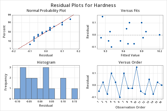{#fig-residualhardness .mx-auto .d-block .lightbox fig-alt="Residual plots for the hardness data showing the normal probability plot, versus fits, residual, and observation order plots" width="60%"}
### Comparing the CRD to the RCBD {.unnumbered .unlisted}
To compare the results from the RCBD, we take a look at the table below. What we did here was use the one-way analysis of variance instead of the two-way to illustrate what might have occurred if we had not blocked, if we had ignored the variation due to the different specimens.
::: minitab_output
### One-way ANOVA: Hardness versus Tip {.unnumbered .unlisted}
#### Factor Information
| Factor | Levels | Values |
|--------|-------:|------------|
| Tip | 4 | 1, 2, 3, 4 |
: {.w-auto .table-sm .table-responsive .row-header }
#### Analysis of Variance
| Source | DF | Seq SS | Contribution | Adj SS | Adj MS | F-Value | P-Value |
|--------|----:|-------:|-------------:|-------:|--------:|--------:|--------:|
| Tip | 3 | 0.3850 | 29.84% | 0.3850 | 0.12833 | 1.70 | 0.220 |
| Error | 12 | 0.9050 | 70.16% | 0.9050 | 0.07542 | | |
| Total | 15 | 1.2900 | 100.00% | | | | |
: {.w-auto .table-sm .table-responsive .row-header}
#### Model Summary
| S | R-sq | R-sq(adj) | PRESS | R-sq(pred) |
|---------:|-------:|----------:|--------:|-----------:|
| 0.274621 | 29.84% | 12.31% | 1.60889 | 0.00% |
: {.w-auto .table-sm .table-responsive}
:::
This isn't quite fair because we did in fact block, but putting the data into one-way analysis we see the same variation due to tip, which is 3.85. So we are explaining the same amount of variation due to the tip. That has not changed. But now we have 12 degrees of freedom for error because we have not blocked and the sum of squares for error is much larger than it was before, thus our *F*-test is 1.7. If we hadn't blocked the experiment our error would be much larger and in fact, we would not even show a significant difference among these tips. This provides a good illustration of the benefit of blocking to reduce error. Notice that the standard deviation, $S=\sqrt{MSE},$ would be about three times larger if we had not blocked.
### Other Aspects of the RCBD {.unnumbered .unlisted}
The RCBD utilizes an **additive model** – one in which there is no interaction between treatments and blocks. *The error term in a randomized complete block model reflects how the treatment effect varies from one block to another.*
Both the treatments and blocks can be looked at as random effects rather than fixed effects, if the levels were selected at random from a population of possible treatments or blocks. We consider this case later, but it does not change the test for a treatment effect.
What are the **consequences** of **not blocking** if we should have? Generally the unexplained error in the model will be larger, and therefore the test of the treatment effect less powerful.
**How to determine the sample size** in the RCBD? The **OC curve** approach can be used to determine the number of blocks to run. The number of blocks, ***b***, represents the number of replications. The power calculations that we looked at before would be the same, except that we use *b* rather than *n*, and we use the estimate of error, $\sigma^2$, that reflects the improved precision based on having used blocks in our experiment. So, the major benefit or power comes not from the number of replications but from the error variance which is much smaller because you removed the effects due to block.
## RCBD and RCBD's with Missing Data
::::::: {#exm-vasculargraft}
### Vascular Graft
\
This example investigates a procedure to create artificial arteries using a resin. The resin is pressed or extruded through an aperture that forms the resin into a tube.
To conduct this experiment as a RCBD, we need to assign all 4 pressures at random to each of the 6 batches of resin. Each batch of resin is called a “**block**”, since a batch is a more homogenous set of experimental units on which to test the extrusion pressures. Below is a table which provides percentages of those products that met the specifications.
::: {#tbl-vascular}
```{=html}
<table align="center" class="table w-auto mx-auto table-sm table-responsive" data-quarto-disable-processing="false" id=#tbl-vascular>
<thead>
<tr>
<th rowspan="2">Extrusion Pressure (PSI)</th>
<th class="text-center" colspan="6">Batch of Resin (Block)</th>
<th class="text-end" rowspan="2">Treatment Total</th>
</tr>
<tr>
<th class="text-center">1</th>
<th class="text-center">2</th>
<th class="text-center">3</th>
<th class="text-center">4</th>
<th class="text-center">5</th>
<th class="text-center">6</th>
</tr>
</thead>
<tbody>
<tr>
<td>8500</td>
<td class="text-center">90.3</td>
<td class="text-center">89.2</td>
<td class="text-center">98.2</td>
<td class="text-center">93.9</td>
<td class="text-center">87.4</td>
<td class="text-center">97.9</td>
<td class="text-end">556.9</td>
</tr>
<tr>
<td>8700</td>
<td class="text-center">92.5</td>
<td class="text-center">89.5</td>
<td class="text-center">90.6</td>
<td class="text-center">94.7</td>
<td class="text-center">87.0</td>
<td class="text-center">95.8</td>
<td class="text-end">550.1</td>
</tr>
<tr>
<td>8900</td>
<td class="text-center">85.5</td>
<td class="text-center">90.8</td>
<td class="text-center">89.6</td>
<td class="text-center">86.2</td>
<td class="text-center">88.0</td>
<td class="text-center">93.4</td>
<td class="text-end">533.5</td>
</tr>
<tr>
<td>9100</td>
<td class="text-center">82.5</td>
<td class="text-center">89.5</td>
<td class="text-center">85.6</td>
<td class="text-center">87.4</td>
<td class="text-center">78.9</td>
<td class="text-center">90.7</td>
<td class="text-end">514.6</td>
</tr>
<tr>
<td>Block Totals</td>
<td class="text-center">350.8</td>
<td class="text-center">359.0</td>
<td class="text-center">364.0</td>
<td class="text-center">362.2</td>
<td class="text-center">341.3</td>
<td class="text-center">377.8</td>
<td class="text-end">\(y_n = 2155.1\)</td>
</tr>
</tbody>
</table>
```
Randomized Complete Block Design for the Vascular Graft Experiment
:::
::: {.callout-caution appearance="minimal"}
**Note!**\
Since percent response data does not generally meet the assumption of constant variance, we might consider a variance stabilizing transformation, i.e., the arcsine square root of the proportion. However, since the range of the percent data is quite limited, it goes from the high 70s through the 90s, this data seems fairly homogeneous.
:::
Output...
::: minitab_output
### Response: Yield {.unnumbered .unlisted}
#### ANOVA for selected Factorial Model
#### Analysis of variance table \[Partial sum of square\]
| Source | Sum of Squares | DF | Mean Square | F Value | Prob \> F |
|----------:|---------------:|----:|------------:|--------:|----------:|
| Block | 192.25 | 5 | 38.45 | | |
| Model | 178.17 | 3 | 59.39 | 8.11 | 0.0019 |
| A | 178.17 | 3 | 59.39 | 8.11 | 0.0019 |
| Residual | 109.89 | 15 | 7.33 | | |
| Cor Total | 480.31 | 23 | | | |
: {.w-auto .table-sm .table-responsive .row-header}
| | | | |
|-----------|-------:|---------------:|-------:|
| Std. Dev. | 2.71 | R-Squared | 0.6185 |
| Mean | 89.80 | Adj R-Squared | 0.5422 |
| C.V. | 3.01 | Pred R-Squared | 0.0234 |
| PRESS | 281.31 | Adeq Precision | 9.759 |
: {.w-auto .table-sm .table-responsive .row-header}
:::
Notice that Design Expert does not perform the hypothesis test on the block factor. Should we test the block factor?
Below is the Minitab output which treats both batch and treatment the same and tests the hypothesis of no effect.
::: minitab_output
### ANOVA: Yield versus Batch, Pressure {.unnumbered .unlisted}
#### Factor Information
| Factor | Type | Levels | Values |
|----------|--------|-------:|------------------------|
| Batch | Random | 6 | 1, 2, 3, 4, 5, 6 |
| Pressure | Fixed | 4 | 8500, 8700, 8900, 9100 |
: {.w-auto .table-sm .table-responsive .row-header}
#### Analysis of Variance for Yield
| Source | DF | SS | MS | F | P |
|----------|----:|------:|-------:|-----:|------:|
| Batch | 5 | 192.3 | 38.450 | 5.25 | 0.006 |
| Pressure | 3 | 178.2 | 59.390 | 8.11 | 0.002 |
| Error | 15 | 109.9 | 7.326 | | |
| Total | 23 | 480.3 | | | |
: {.w-auto .table-sm .table-responsive .row-header}
:::
This example shows the output from the ANOVA command in Minitab (**Menu** \> **Stat** \> **ANOVA** \> **Balanced ANOVA**). It does hypothesis tests for both batch and pressure, and they are both significant. Otherwise, the results from both programs are very similar.
**Again, should we test the block factor?**
Generally, the answer is no, but in some instances, this might be helpful. We use the RCBD design because we hope to remove from error the variation due to the block. If the block factor is not significant, then the block variation, or mean square due to the block treatments is no greater than the mean square due to the error. In other words, if the block *F* ratio is close to 1 (or generally not greater than 2), you have wasted effort in doing the experiment as a block design, **and** used in this case 5 degrees of freedom that could be part of error degrees of freedom, hence the design could actually be less efficient!
Therefore, one can test the block simply to confirm that the block factor is effective and explains variation that would otherwise be part of your experimental error. However, you generally cannot make any stronger conclusions from the test on a block factor, because you may not have randomly selected the blocks from any population, nor randomly assigned the levels.
**Why did I first say no?**
There are two cases we should consider separately when blocks are: 1) a classification factor and 2) an experimental factor. In the case where blocks are a batch, it is a classification factor, but it might also be subjects or plots of land which are also classification factors. For a RCBD you can apply your experiment to convenient subjects. In the general case of classification factors, you should sample from the population in order to make inferences about that population. These observed batches are not necessarily a sample from any population. If you want to make inferences about a factor then there should be an appropriate randomization, i.e. random selection, so that you can make inferences about the population. In the case of experimental factors, such as oven temperature for a process, all you want is a representative set of temperatures such that the treatment is given under homogeneous conditions. The point is that we set the temperature once in each block; we don't reset it for each observation. So, there is no replication of the block factor. We do our randomization of treatments within a block. In this case, there is an asymmetry between treatment and block factors. In summary, you are only including the block factor to reduce the error variation due to this nuisance factor, not to test the effect of this factor.
:::::::
### ANOVA: Yeild versus Batch, Pressure {.unnumbered .unlisted}
The residual analysis for the Vascular Graft example is shown: 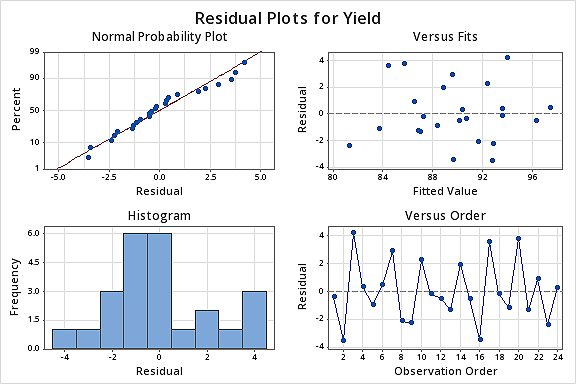{#fig-yieldbatch4in1graphs .mx-auto .d-block .lightbox fig-alt="Residual plots showing the normal probability plot, the residuals versus fits, the histogram of the residuals and the residuals versus the order " width="60%"}
The pattern does not strike me as indicating an unequal variance.
Another way to look at these residuals is to plot the residuals against the two factors. Notice that pressure is the treatment factor and batch is the block factor. Here we'll check for homogeneous variance. Against treatment these look quite homogeneous.
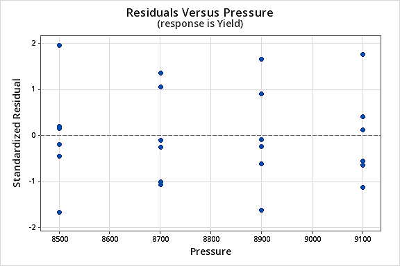{#fig-residualvspressure .mx-auto .d-block .lightbox fig-alt="Residual plot where the response is Yield versus Pressure" width="60%"}
Plotted against block the sixth does raise ones eyebrow a bit. It seems to be very close to zero.
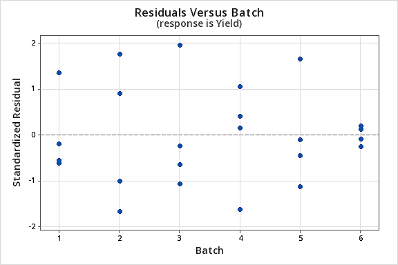{#fig-residualvsbatch .mx-auto .d-block .lightbox fig-alt="Residual plot where the response is Yield versus Batch" width="60%"}
Basic residual plots indicate that **normality**, **constant variance** assumptions are satisfied. Therefore, there seems to be no obvious problems with **randomization.** These plots provide more information about the constant variance assumption, and can reveal possible outliers. The plot of residuals versus order sometimes indicates a problem with the independence assumption.
### Missing Data {.unnumbered .unlisted}
In the example dataset above, what if the data point 94.7 (second treatment, fourth block) was missing? What data point can I substitute for the missing point?
If this point is missing we can substitute *x*, calculate the sum of squares residuals, and solve for *x* which minimizes the error and gives us a point based on all the other data and the two-way model. We sometimes call this an imputed point, where you use the least squares approach to estimate this missing data point.
After calculating *x*, you could substitute the estimated data point and repeat your analysis. Now you have an artificial point with known residual zero. So you can analyze the resulting data, but now should reduce your error degrees of freedom by one. In any event, these are all approximate methods, i.e., using the best fitting or imputed point.
Before high-speed computing, data imputation was often done because the ANOVA computations are more readily done using a balanced design. There are times where imputation is still helpful but in the case of a two-way or multiway ANOVA we generally will use the General Linear Model (GLM) and use the full and reduced model approach to do the appropriate test. This is often called the General Linear Test (GLT).
Let's take a look at this in Minitab now (no sound)...
::: {#vid-missingdata}
::: text-center
```{=html}
<iframe id="kaltura_player_1789320299" src="https://cdnapisec.kaltura.com/p/2356971/embedPlaykitJs/uiconf_id/56368382?iframeembed=true&entry_id=1_ho5jt276&config[provider]=%7B%22widgetId%22%3A%221_2y9oqq18%22%7D" width="100%" height="690" allowfullscreen webkitallowfullscreen mozAllowFullScreen allow="autoplay *; fullscreen *; encrypted-media *" style="position:relative;top:0;left:0;width:95%;height:640px;border:0"></iframe>
```
:::
:::
The sum of squares you want to use to test your hypothesis will be based on the adjusted treatment sum of squares, $R( \tau_i | \mu, \beta_j)$ using the notation for testing:
$H_0 \colon \tau_i = 0$
The numerator of the F-test, for the hypothesis you want to test, should be based on the adjusted SS's that is last in the sequence or is obtained from the adjusted sums of squares. That will be very close to what you would get using the approximate method we mentioned earlier. The general linear test is the most powerful test for this type of situation with unbalanced data.
The General Linear Test can be used to test for significance of multiple parameters of the model at the same time. Generally, the significance of all those parameters which are in the Full model but are not included in the Reduced model are tested, simultaneously. The F test statistic is defined as
$$F^\ast=\dfrac{SSE(R)-SSE(F)}{df_R-df_F}\div \dfrac{SSE(F)}{df_F}$$
Where F stands for “Full” and R stands for “Reduced.” The numerator and denominator degrees of freedom for the F statistic is $df_R - df_F$ and $df_F$ , respectively.
Here are the results for the GLM with all the data intact. There are 23 degrees of freedom total here so this is based on the full set of 24 observations.
::: minitab_output
### General Linear Model: Yield versus Batch, Pressure {.unnumbered .unlisted}
#### Factor Information
| Factor | Type | Levels | Values |
|:---------|--------|-------:|------------------------|
| Batch | Random | 6 | 1, 2, 3, 4, 5, 6 |
| Pressure | Fixed | 4 | 8500, 8700, 8900, 9100 |
: {.w-auto .table-sm .table-responsive .row-header}
#### Analysis of Variance for Yield
| Source | DF | SS | MS | F | P |
|:---------|----:|------:|-------:|-----:|------:|
| Batch | 5 | 192.3 | 38.450 | 5.25 | 0.006 |
| Pressure | 3 | 178.2 | 59.390 | 8.11 | 0.002 |
| Error | 15 | 109.9 | 7.326 | | |
| Total | 23 | 480.3 | | | |
: {.w-auto .table-sm .table-responsive .row-header}
#### Model Summary
| S | R-sq | R-sq(adj) | R-sq(pred) |
|--------:|-------:|----------:|-----------:|
| 2.70661 | 77.12% | 64.92% | 41.43% |
: {.w-auto .table-sm .table-responsive .row-header}
#### Least Squares Means for Yield
| Pressure | Mean | SE Mean |
|:---------|------:|--------:|
| 8500 | 92.82 | 1.105 |
| 8700 | 91.68 | 1.105 |
| 8900 | 88.92 | 1.105 |
| 9100 | 85.77 | 1.105 |
: {.w-auto .table-sm .table-responsive .row-header}
[Main Effects Plot (fitted means) for Yield]{.small}
:::
When the data are complete this analysis from GLM is correct and equivalent to the results from the two-way command in Minitab. When you have missing data, the raw marginal means are wrong. What if the missing data point were from a very high measuring block? It would reduce the overall effect of that treatment, and the estimated treatment mean would be biased.
Above you have the least squares means that correspond exactly to the simple means from the earlier analysis.
We now illustrate the GLM analysis based on the missing data situation - one observation missing (Batch 4, pressure 2 data point removed). The least squares means as you can see (below) are slightly different, for pressure 8700. What you also want to notice is the standard error of these means, i.e., the S.E., for the second treatment is slightly larger. The fact that you are missing a point is reflected in the estimate of error. You do not have as many data points on that particular treatment.
::: minitab_output
### General Linear Model: Yield versus Batch, Pressure {.unnumbered .unlisted}
#### Factor Information
| Factor | Type | Levels | Values |
|:---------|--------|-------:|------------------------|
| Batch | Random | 6 | 1, 2, 3, 4, 5, 6 |
| Pressure | Fixed | 4 | 8500, 8700, 8900, 9100 |
: {.w-auto .table-sm .table-responsive .row-header}
#### Analysis of Variance
| Source | DF | Adj SS | Adj MS | F-Value | P-Value |
|----------|----:|-------:|-------:|--------:|--------:|
| Batch | 5 | 189.5 | 37.904 | 5.22 | 0.007 |
| Pressure | 3 | 163.4 | 54.466 | 7.50 | 0.003 |
| Error | 14 | 101.7 | 7.264 | | |
| Total | 22 | 455.2 | | | |
: {.w-auto .table-sm .table-responsive .row-header}
#### Model Summary
| S | R-sq | R-sq(adj) | R-sq(pred) |
|--------:|-------:|----------:|-----------:|
| 2.69518 | 77.66% | 64.89% | 39.92% |
: {.w-auto .table-sm .table-responsive .row-header}
#### Least Squares Means for Yield
| Pressure | Mean | SE Mean |
|:---------|------:|--------:|
| 8500 | 92.82 | 1.105 |
| 8700 | 91.08 | 1.238 |
| 8900 | 88.92 | 1.105 |
| 9100 | 85.77 | 1.105 |
: {.w-auto .table-sm .table-responsive .row-header}
[Main Effects Plot (fitted means) for Yield]{.small}
:::
The overall results are similar. We have only lost one point and our hypothesis test is still significant, with a p-value of 0.003 rather than 0.002.
Here is a plot of the least squares means for Yield with all of the observations included.
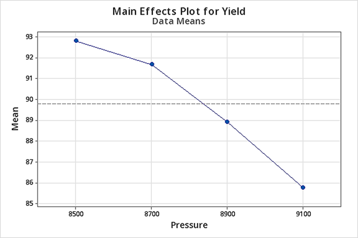{#fig-maineffectsplotfull .mx-auto .d-block .lightbox fig-alt="Main effects plot showing mean vs pressure for Yield with all data" width="60%"}
Here is a plot of the least squares means for Yield with the missing data, not very different.
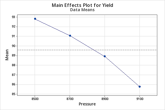{#fig-maineffectsplotmiss .mx-auto .d-block .lightbox fig-alt="Main effects plot showing mean vs pressure for Yield with missing one data point" width="60%"}
Again, for any unbalanced data situation, we will use the GLM. For most of our examples, GLM will be a useful tool for analyzing and getting the analysis of variance summary table. Even if you are unsure whether your data are orthogonal, one way to check if you simply made a mistake in entering your data is by checking whether the sequential sums of squares agree with the adjusted sums of squares.
## The Latin Square Design
Latin Square Designs are probably not used as much as they should be - they are very efficient designs. Latin square designs allow for two blocking factors. In other words, these designs are used to simultaneously control (or eliminate) **two sources of nuisance variability**. For instance, if you had a plot of land the fertility of this land might change in both directions, North -- South and East -- West due to soil or moisture gradients. So, both rows and columns can be used as blocking factors. However, you can use Latin squares in lots of other settings. As we shall see, Latin squares can be used as much as the RCBD in industrial experimentation as well as other experiments.
Whenever, you have more than one blocking factor a Latin square design will allow you to remove the variation for these two sources from the error variation. So, consider we had a plot of land, we might have blocked it in columns and rows, i.e. each row is a level of the row factor, and each column is a level of the column factor. We can remove the variation from our measured response in both directions if we consider both rows and columns as factors in our design.
The Latin Square Design gets its name from the fact that we can write it as a square with Latin letters to correspond to the treatments. The treatment factor levels are the Latin letters in the Latin square design. The number of rows and columns has to correspond to the number of treatment levels. So, if we have four treatments then we would need to have four rows and four columns in order to create a Latin square. This gives us a design where we have each of the treatments and in each row and in each column.
::: {#fig-latinsquare1 .bg-white .w-50 .mx-auto .d-block .mb-3}
```{=html}
<svg id="svg2" role="img" viewbox="0 0 212.87 136.67" xmlns="http://www.w3.org/2000/svg" aria-labelledby="title"><title>Latin suqare showing how each treatment A occurs in every column and row</title><g data-name="Layer 2" fill="none" stroke="#000" stroke-miterlimit="10"><path d="M22.24 14.17h122v122h-122z"></path><path d="M53.6 14.17v122M83.6 14.17v122M113.6 14.17v121.54M22.24 45.03h122M22.24 75.03h122M22.24 105.33l122-.08" stroke-width=".75"></path></g><g data-name="Layer 3"><text font-family="Calibri, Arial" font-size="12" font-weight="600" transform="translate(66.82 10.28)">columns</text><text font-family="Calibri, Arial" font-size="12" font-weight="600" transform="rotate(-90 48.075 37.795)">rows</text><circle cx="39.31" cy="28.49" fill="#fdedc4" r="10.81"></circle><text fill="#065094" font-family="Calibri, Arial" font-size="16" font-weight="600" transform="translate(34.02 34.31)">A</text><text fill="#065094" font-family="Calibri, Arial" font-size="16" font-weight="600" transform="translate(62.49 35.22)">B</text><text fill="#065094" font-family="Calibri, Arial" font-size="16" font-weight="600" transform="translate(93.25 34.68)">C</text><text fill="#065094" font-family="Calibri, Arial" font-size="16" font-weight="600" transform="translate(122.75 35.25)">D</text><text fill="#065094" font-family="Calibri, Arial" font-size="16" font-weight="600" transform="translate(33.36 66.57)">B</text><text fill="#065094" font-family="Calibri, Arial" font-size="16" font-weight="600" transform="translate(122.96 95.75)">B</text><text fill="#065094" font-family="Calibri, Arial" font-size="16" font-weight="600" transform="translate(92.95 127.25)">B</text><text fill="#065094" font-family="Calibri, Arial" font-size="16" font-weight="600" transform="translate(62.95 66.52)">C</text><text fill="#065094" font-family="Calibri, Arial" font-size="16" font-weight="600" transform="translate(33.81 95.75)">C</text><text fill="#065094" font-family="Calibri, Arial" font-size="16" font-weight="600" transform="translate(123.31 127.08)">C</text><text fill="#065094" font-family="Calibri, Arial" font-size="16" font-weight="600" transform="translate(92.74 66.77)">D</text><text fill="#065094" font-family="Calibri, Arial" font-size="16" font-weight="600" transform="translate(62.28 95.41)">D</text><text fill="#065094" font-family="Calibri, Arial" font-size="16" font-weight="600" transform="translate(33.14 126.91)">D</text><text font-family="Calibri, Arial" font-size="12" font-weight="600" transform="translate(150.55 39.05)">Each <tspan x="0" y="14.4">treatment </tspan><tspan x="0" y="28.8">occurs in </tspan><tspan x="0" y="43.2">every </tspan><tspan x="0" y="57.6">column </tspan><tspan x="0" y="72">and row</tspan></text><circle cx="128.74" cy="61.66" fill="#fdedc4" r="10.81"></circle><text fill="#065094" font-family="Calibri, Arial" font-size="16" font-weight="600" transform="translate(123.45 67.48)">A</text><circle cx="98.74" cy="89.76" fill="#fdedc4" r="10.81"></circle><text fill="#065094" font-family="Calibri, Arial" font-size="16" font-weight="600" transform="translate(93.45 95.58)">A</text><circle cx="68.02" cy="121.26" fill="#fdedc4" r="10.81"></circle><text fill="#065094" font-family="Calibri, Arial" font-size="16" font-weight="600" transform="translate(62.73 127.08)">A</text></g></svg>
```
:::
This is just one of many 4×4 squares that you could create. In fact, you can make any size square you want, for any number of treatments - it just needs to have the following property associated with it - that each treatment occurs only once in each row and once in each column.
Consider another example in an industrial setting: the rows are the batch of raw material, the columns are the operator of the equipment, and the treatments (A, B, C and D) are an industrial process or protocol for producing a particular product.
What is the model? We let:
$$y_{ijk} = \mu + \rho_i + \beta_j + \tau_k + e_{ijk}$$
$i = 1, ... , t$ $j = 1, ... , t$ \[$k = 1, ... , t$\] where - $k = d(i, j)$ and the total number of observations
$N = t^2$ (the number of rows times the number of columns) and *t* is the number of treatments.
Note that a Latin Square is an incomplete design, which means that it does not include observations for all possible combinations of i,*j* and k. This is why we use notation $k = d(i, j)$. Once we know the row and column of the design, then the treatment is specified. In other words, if we know *i* and *j*, then *k* is specified by the Latin Square design.
This property has an impact on how we calculate means and sums of squares, and for this reason, we can not use the balanced ANOVA command in Minitab even though it looks perfectly balanced. We will see later that although it has the property of orthogonality, you still cannot use the balanced ANOVA command in Minitab because it is not complete.
An assumption that we make when using a Latin square design is that the three factors (treatments, and two nuisance factors) do not interact. If this assumption is violated, the Latin Square design error term will be inflated.
The randomization procedure for assigning treatments that you would like to use when you actually apply a Latin Square, is somewhat restricted to preserve the structure of the Latin Square. The ideal randomization would be to select a square from the set of all possible Latin squares of the specified size. However, a more practical randomization scheme would be to select a standardized Latin square at random (these are tabulated) and then:
1. randomly permute the columns,
2. randomly permute the rows, and then
3. assign the treatments to the Latin letters in a random fashion.
Consider a factory setting where you are producing a product with 4 operators and 4 machines. We call the columns the operators and the rows the machines. Then you can randomly assign the specific operators to a row and the specific machines to a column. The treatment is one of four protocols for producing the product and our interest is in the average time needed to produce each product. If both the machine and the operator have an effect on the time to produce, then by using a Latin Square Design this variation due to machine or operators will be effectively removed from the analysis.
The following table gives the degrees of freedom for the terms in the model.
| AOV | df | df for the example |
|:-----------|-------------:|-------------------:|
| Rows | $t-1$ | 3 |
| Cols | $t-1$ | 3 |
| Treatments | $t-1$ | 3 |
| Error | $(t-1)(t-2)$ | 6 |
| Total | ($t^2 - 1$) | 15 |
: {.w-auto .table-sm .table-responsive .mx-auto .row-header}
A Latin Square design is actually easy to analyze. Because of the restricted layout, one observation per treatment in each row and column, the model is orthogonal.
If the row, $\rho_i$, and column, $\beta_j$, effects are random with expectations zero, the expected value of $Y_{ijk}$ is $\mu + \tau_k$. In other words, the treatment effects and treatment means are orthogonal to the row and column effects. We can also write the sums of squares, as seen in Table 4.10 in the text.
We can test for row and column effects, but our focus of interest in a Latin square design is on the treatments. Just as in RCBD, the row and column factors are included to reduce the error variation but are not typically of interest. And, depending on how we've conducted the experiment they often haven't been randomized in a way that allows us to make any reliable inference from those tests.
Note: if you have missing data then you need to use the general linear model and test the effect of treatment after fitting the model that would account for the row and column effects.
In general, the General Linear Model tests the hypothesis that:
$$H_0 \colon \tau_i = 0 \text{ vs. } H_A \colon \tau_i \ne 0$$
To test this hypothesis we will look at the F-ratio which is written as:
$$F=\dfrac{MS(\tau_k|\mu,\rho_i,\beta_j)}{MSE(\mu,\rho_i,\beta_j,\tau_k)}\sim F((t-1),(t-1)(t-2))$$
To get this in Minitab you would use GLM and fit the three terms: rows, columns and treatments. The F statistic is based on the adjusted MS for treatment.
**The Rocket Propellant Problem – A Latin Square Design**
```{=html}
<table align="center" class="table w-auto mx-auto table-sm table-responsive" data-quarto-disable-processing="false"><caption>Latin Square Design for the Rocket Propellant</caption>
<thead>
<tr>
<th></th>
<th class="text-center" colspan="5">Operators</th>
</tr>
<tr>
<th class="text-end">Batches of Raw Material</th>
<th class="text-center" >1</th>
<th class="text-center">2</th>
<th class="text-center">3</th>
<th class="text-center">4</th>
<th class="text-center">5</th>
</tr>
</thead>
<tbody>
<tr>
<td class="text-center">1</td>
<td>A = 24</td>
<td>B = 20</td>
<td>C = 19</td>
<td>D = 24</td>
<td>E = 24</td>
</tr>
<tr>
<td class="text-center">2</td>
<td>B = 17</td>
<td>C = 24</td>
<td>D = 30</td>
<td>E = 27</td>
<td>A = 36</td>
</tr>
<tr>
<td class="text-center">3</td>
<td>C = 18</td>
<td>D = 38</td>
<td>E = 26</td>
<td>A = 27</td>
<td>B = 21</td>
</tr>
<tr>
<td class="text-center">4</td>
<td>D = 26</td>
<td>E = 31</td>
<td>A = 26</td>
<td>B = 23</td>
<td>C = 22</td>
</tr>
<tr>
<td class="text-center">5</td>
<td>E = 22</td>
<td>A = 30</td>
<td>B = 20</td>
<td>C = 29</td>
<td>D = 31</td>
</tr>
<tr>
<td></td>
<td></td>
<td></td>
<td></td>
<td></td>
<td></td>
</tr>
</tbody>
</table>
```
### Statistical Analysis of the Latin Square Design {.unnumbered .unlisted}
The statistical (effects) model is:
$$Y_{ijk}=\mu +\rho_i+\beta_j+\tau_k+\varepsilon_{ijk}
\left\{\begin{array}{c}
i=1,2,\ldots,p \\
j=1,2,\ldots,p\\
k=1,2,\ldots,p
\end{array}\right. $$
but $k = d(i, j)$ shows the dependence of *k* in the cell *i*, *j* on the design layout, and *p = t* the number of treatment levels.
The statistical analysis (ANOVA) is much like the analysis for the RCBD.
The analysis for the rocket propellant example is presented in Example 4.3.
## Replicated Latin Squares
Latin Squares are very efficient by including two blocking factors, however, the *d.f.* for error are often too small. In these situations, we consider replicating a Latin Square. Let's go back to the factory scenario again as an example and look at $n = 3$ repetitions of a 4 × 4 Latin square.
We labeled the row factor the machines, the column factor the operators and the Latin letters denoted the protocol used by the operators which were the treatment factor. We will replicate this Latin Square experiment $n = 3$ times. Now we have total observations equal to $N = t^{2}$.
You could use the same squares over again in each replicate, but we prefer to randomize these separately for each replicate. It might look like this:
::: {#fig-latinsquare3operators .bg-white .w-75 .mx-auto .d-block .mb-3}
```{=html}
<svg data-name="Layer 3" viewbox="0 0 522.31 196.92" xmlns="http://www.w3.org/2000/svg" id="svg2" role="img" aria-labelledby="title" > <title>3 difference Latin Squares for 3 reps </title> <path d="M19.96 25.37h151.35v151.35H19.96z" fill="none" stroke="#000" stroke-miterlimit="10" stroke-width="2"></path> <path d="M58.53 25.54v151.35M95.64 25.37v151.36M132.61 25.37v150.79M19.96 63.66h151.35M19.96 100.74h151.35M19.96 138.7l151.35-.11" fill="none" stroke="#000" stroke-miterlimit="10" stroke-width=".75"></path> <text font-size="12" transform="translate(12.2 49.69)"> 1 </text> <text font-size="12" transform="translate(12.2 87.19)"> 2 </text> <text font-size="12" transform="translate(12.2 124.69)"> 3 </text> <text font-size="12" transform="translate(12.2 162.19)"> 4 </text> <text font-size="12" transform="translate(37.49 23.26)"> 1 </text> <text font-size="12" transform="translate(74.23 23.26)"> 2 </text> <text font-size="12" transform="translate(110.97 23.26)"> 3 </text> <text font-size="12" transform="translate(147.71 23.26)"> 4 </text> <text font-size="12" transform="rotate(-90 67.55 57.51)"> machines </text> <text font-size="12" transform="translate(71.85 10.15)"> operators </text> <text font-size="12" transform="translate(83.85 193.92)"> <tspan letter-spacing="0em">Rep 1</tspan> </text> <text fill="#065094" font-size="16" transform="translate(34.67 50.18)"> A </text> <text fill="#065094" font-size="16" transform="translate(71.17 50.35)"> B </text> <text fill="#065094" font-size="16" transform="translate(108.12 50.35)"> C </text> <text fill="#065094" font-size="16" transform="translate(144.93 50)"> D </text> <text fill="#065094" font-size="16" transform="translate(146.03 88.6)"> A </text> <text fill="#065094" font-size="16" transform="translate(108.26 125.81)"> A </text> <text fill="#065094" font-size="16" transform="translate(71.76 163.77)"> A </text> <text fill="#065094" font-size="16" transform="translate(34.26 89.77)"> B </text> <text fill="#065094" font-size="16" transform="translate(146.14 124.99)"> B </text> <text fill="#065094" font-size="16" transform="translate(107.74 163.94)"> B </text> <text fill="#065094" font-size="16" transform="translate(71.49 88.77)"> C </text> <text fill="#065094" font-size="16" transform="translate(34.16 125.99)"> C </text> <text fill="#065094" font-size="16" transform="translate(146.06 163.94)"> C </text> <text fill="#065094" font-size="16" transform="translate(108.19 88.42)"> D </text> <text fill="#065094" font-size="16" transform="translate(71.76 125.64)"> D </text> <text fill="#065094" font-size="16" transform="translate(34.71 163.59)"> D </text> <text font-size="12" transform="rotate(-90 154.405 -29.785)"> machines </text> <path d="M194.96 25.27h151.35v151.35H194.96z" fill="none" stroke="#000" stroke-miterlimit="10" stroke-width="2"></path> <path d="M233.53 25.43v151.36M270.64 25.27v151.35M307.61 25.27v150.79M194.96 63.56h151.35M194.96 100.64h151.35M194.96 138.59l151.35-.1" fill="none" stroke="#000" stroke-miterlimit="10" stroke-width=".75"></path> <text font-size="12" transform="translate(187.2 49.59)"> 1 </text> <text font-size="12" transform="translate(187.2 87.09)"> 2 </text> <text font-size="12" transform="translate(187.2 124.59)"> 3 </text> <text font-size="12" transform="translate(187.2 162.09)"> 4 </text> <text font-size="12" transform="translate(212.49 23.15)"> 1 </text> <text font-size="12" transform="translate(249.23 23.15)"> 2 </text> <text font-size="12" transform="translate(285.97 23.15)"> 3 </text> <text font-size="12" transform="translate(322.71 23.15)"> 4 </text> <text font-size="12" transform="translate(246.85 10.04)"> operators </text> <text font-size="12" transform="translate(259.85 193.82)"> <tspan letter-spacing="0em">Rep 2</tspan> </text> <text fill="#065094" font-size="16" transform="translate(209.28 51.57)"> D </text> <text fill="#065094" font-size="16" transform="translate(246.59 52.57)"> A </text> <text fill="#065094" font-size="16" transform="translate(283.76 52.1)"> B </text> <text fill="#065094" font-size="16" transform="translate(320.21 52.23)"> C </text> <text fill="#065094" font-size="16" transform="translate(209.67 86.57)"> A </text> <text fill="#065094" font-size="16" transform="translate(246.65 87.57)"> B </text> <text fill="#065094" font-size="16" transform="translate(283.76 87.1)"> C </text> <text fill="#065094" font-size="16" transform="translate(319.93 87.23)"> D </text> <text fill="#065094" font-size="16" transform="translate(208.5 124.73)"> B </text> <text fill="#065094" font-size="16" transform="translate(246.54 125.74)"> C </text> <text fill="#065094" font-size="16" transform="translate(283.46 125.26)"> D </text> <text fill="#065094" font-size="16" transform="translate(320.76 125.39)"> A </text> <text fill="#065094" font-size="16" transform="translate(208.89 162.14)"> C </text> <text fill="#065094" font-size="16" transform="translate(246.02 162.47)"> D </text> <text fill="#065094" font-size="16" transform="translate(283.46 162.66)"> A </text> <text fill="#065094" font-size="16" transform="translate(320.48 162.79)"> B </text> <path d="M369.96 25.27h151.35v151.35H369.96z" fill="none" stroke="#000" stroke-miterlimit="10" stroke-width="2"></path> <path d="M408.53 25.43v151.36M445.64 25.27v151.35M482.61 25.27v150.79M369.96 63.56h151.35M369.96 100.64h151.35M369.96 138.59l151.35-.1" fill="none" stroke="#000" stroke-miterlimit="10" stroke-width=".75"></path> <text font-size="12" transform="translate(362.2 49.59)"> 1 </text> <text font-size="12" transform="translate(362.2 87.09)"> 2 </text> <text font-size="12" transform="translate(362.2 124.59)"> 3 </text> <text font-size="12" transform="translate(362.2 162.09)"> 4 </text> <text font-size="12" transform="translate(387.49 23.15)"> 1 </text> <text font-size="12" transform="translate(424.23 23.15)"> 2 </text> <text font-size="12" transform="translate(460.97 23.15)"> 3 </text> <text font-size="12" transform="translate(497.71 23.15)"> 4 </text> <text font-size="12" transform="rotate(-90 243.135 -118.075)"> machines </text> <text font-size="12" transform="translate(421.85 10.04)"> operators </text> <text font-size="12" transform="translate(434.85 193.82)"> <tspan letter-spacing="0em">Rep 3</tspan> </text> <text fill="#065094" font-size="16" transform="translate(383.29 51.7)"> C </text> <text fill="#065094" font-size="16" transform="translate(419.97 52.2)"> D </text> <text fill="#065094" font-size="16" transform="translate(458.32 51.22)"> A </text> <text fill="#065094" font-size="16" transform="translate(495.21 52.35)"> B </text> <text fill="#065094" font-size="16" transform="translate(383.1 89.57)"> D </text> <text fill="#065094" font-size="16" transform="translate(419.93 89.57)"> A </text> <text fill="#065094" font-size="16" transform="translate(456.73 90.1)"> B </text> <text fill="#065094" font-size="16" transform="translate(492.93 90.23)"> C </text> <text fill="#065094" font-size="16" transform="translate(383.49 124.73)"> A </text> <text fill="#065094" font-size="16" transform="translate(420.81 124.74)"> B </text> <text fill="#065094" font-size="16" transform="translate(457.79 124.26)"> C </text> <text fill="#065094" font-size="16" transform="translate(494.76 124.39)"> D </text> <text fill="#065094" font-size="16" transform="translate(383.69 162.14)"> B </text> <text fill="#065094" font-size="16" transform="translate(420.71 162.47)"> C </text> <text fill="#065094" font-size="16" transform="translate(458.34 162.66)"> D </text> <text fill="#065094" font-size="16" transform="translate(495.48 161.79)"> A </text> </svg>
```
:::
### Case 1 {.unnumbered .unlisted}
Here we will have the same row and column levels. For instance, we might do this experiment all in the same factory using the same machines and the same operators for these machines. The first replicate would occur during the first week, the second replicate would occur during the second week, etc. Week one would be replication one, week two would be replication two and week three would be replication three.
We would write the model for this case as:
$$Y_{hijk}=\mu +\delta _{h}+\rho _{i}+\beta _{j}+\tau _{k}+e_{hijk}$$
where:
::: ms-3
$h = 1, \dots , n$\
$i = 1, \dots , t$\
$j = 1, \dots , t$\
$k = d_{h}(i,j)$ - the Latin letters
:::
This is a simple extension of the basic model that we had looked at earlier. We have added one more term to our model. The row and column and treatment all have the same parameters, the same effects that we had in the single Latin square. In a Latin square, the error is a combination of any interactions that might exist and experimental error. Remember, we can't estimate interactions in a Latin square.
Let's take a look at the analysis of variance table.
| AOV | df | df for Case 1 | SS |
|:-------------------|:--------------------------------|:--------------|-----|
| rep=week | $n − 1$ | 2 | |
| row=machine | $t − 1$ | 3 | |
| column=operator | $t − 1$ | 3 | |
| treatment=protocol | $t − 1$ | 3 | |
| error | $( t − 1 ) [ n ( t + 1 ) − 3 ]$ | 36 | |
| Total | $n t^ 2 − 1$ | 47 | |
: {.w-auto .table-sm .table-responsive .mx-auto .row-header}
### Case 2 {.unnumbered .unlisted}
In this case, one of our blocking factors, either row or column, is going to be the same across replicates whereas the other will take on new values in each replicate. Back to the factory example e.g., we would have a situation where the machines are going to be different (you can say they are nested in each of the repetitions) but the operators will stay the same (crossed with replicates). In this scenario, perhaps, this factory has three locations and we want to include machines from each of these three different factories. To keep the experiment standardized, we will move our operators with us as we go from one factory location to the next. This might be laid out like this:
::: {#fig-latinsquare3factories .bg-white .w-75 .mx-auto .d-block .mb-3}
```{=html}
<svg data-name="Layer 3" viewbox="0 0 527.03 211.18" xmlns="http://www.w3.org/2000/svg" id="svg2" role="img" aria-labelledby="title" > <title>This image shows three 4x4 replicated Latin squares, representing three repetitions (Rep 1, Rep 2, and Rep 3) across Factory 1, Factory 2, and Factory 3. Each square assigns 4 operators (A, B, C, D) to 4 machines in a way that each operator appears exactly once per row and column. The machines are numbered 1-12 across all three factories, with operators rotated systematically to ensure balanced assignments. </title><path d="M19.96 25.27h151.35v151.35H19.96z" fill="none" stroke="#000" stroke-miterlimit="10" stroke-width="2"></path><path d="M58.53 25.43v151.36M95.63 25.27v151.35M132.61 25.27v150.79M19.96 63.56h151.35M19.96 100.64h151.35M19.96 138.59l151.35-.1" fill="none" stroke="#000" stroke-miterlimit="10" stroke-width=".75"></path><text font-size="12" transform="translate(12.2 49.59)">1</text><text font-size="12" transform="translate(12.2 87.09)">2</text><text font-size="12" transform="translate(12.2 124.59)">3</text><text font-size="12" transform="translate(12.2 162.09)">4</text><text font-size="12" transform="translate(37.49 23.15)">1</text><text font-size="12" transform="translate(74.23 23.15)">2</text><text font-size="12" transform="translate(110.97 23.15)">3</text><text font-size="12" transform="translate(147.71 23.15)">4</text><text font-size="12" transform="rotate(-90 67.5 57.46)">machines</text><text font-size="12" transform="translate(71.85 10.04)">operators</text><text font-size="12" transform="translate(83.85 193.82)"><tspan letter-spacing="0em">Rep 1</tspan></text><text fill="#065094" font-size="16" transform="translate(34.67 50.07)">A</text><text fill="#065094" font-size="16" transform="translate(71.17 50.25)">B</text><text fill="#065094" font-size="16" transform="translate(108.12 50.25)">C</text><text fill="#065094" font-size="16" transform="translate(144.93 49.9)">D</text><text fill="#065094" font-size="16" transform="translate(146.03 88.49)">A</text><text fill="#065094" font-size="16" transform="translate(108.26 125.71)">A</text><text fill="#065094" font-size="16" transform="translate(71.76 163.66)">A</text><text fill="#065094" font-size="16" transform="translate(34.26 89.67)">B</text><text fill="#065094" font-size="16" transform="translate(146.14 124.88)">B</text><text fill="#065094" font-size="16" transform="translate(107.73 163.84)">B</text><text fill="#065094" font-size="16" transform="translate(71.49 88.67)">C</text><text fill="#065094" font-size="16" transform="translate(34.16 125.88)">C</text><text fill="#065094" font-size="16" transform="translate(146.06 163.84)">C</text><text fill="#065094" font-size="16" transform="translate(108.19 88.32)">D</text><text fill="#065094" font-size="16" transform="translate(71.76 125.54)">D</text><text fill="#065094" font-size="16" transform="translate(34.71 163.49)">D</text><text font-size="12" transform="translate(73.05 207.43)"><tspan letter-spacing="-.05em">Factory 1</tspan></text><text font-size="12" transform="rotate(-90 155.505 -30.035)">machines</text><path d="M194.96 25.27h151.35v151.35H194.96z" fill="none" stroke="#000" stroke-miterlimit="10" stroke-width="2"></path><path d="M233.53 25.43v151.36M270.63 25.27v151.35M307.61 25.27v150.79M194.96 63.56h151.35M194.96 100.64h151.35M194.96 138.59l151.35-.1" fill="none" stroke="#000" stroke-miterlimit="10" stroke-width=".75"></path><text font-size="12" transform="translate(187.2 49.59)">5</text><text font-size="12" transform="translate(187.2 87.09)">6</text><text font-size="12" transform="translate(187.2 124.59)">7</text><text font-size="12" transform="translate(187.2 162.09)">8</text><text font-size="12" transform="translate(212.49 23.15)">1</text><text font-size="12" transform="translate(249.23 23.15)">2</text><text font-size="12" transform="translate(285.97 23.15)">3</text><text font-size="12" transform="translate(322.71 23.15)">4</text><text font-size="12" transform="translate(246.85 10.04)">operators</text><text font-size="12" transform="translate(259.85 193.82)"><tspan letter-spacing="0em">Rep 2</tspan></text><text fill="#065094" font-size="16" transform="translate(209.28 51.57)">D</text><text fill="#065094" font-size="16" transform="translate(246.59 52.57)">A</text><text fill="#065094" font-size="16" transform="translate(283.76 52.1)">B</text><text fill="#065094" font-size="16" transform="translate(320.2 52.23)">C</text><text fill="#065094" font-size="16" transform="translate(209.67 86.57)">A</text><text fill="#065094" font-size="16" transform="translate(246.65 87.57)">B</text><text fill="#065094" font-size="16" transform="translate(283.76 87.1)">C</text><text fill="#065094" font-size="16" transform="translate(319.93 87.23)">D</text><text fill="#065094" font-size="16" transform="translate(208.5 124.73)">B</text><text fill="#065094" font-size="16" transform="translate(246.54 125.74)">C</text><text fill="#065094" font-size="16" transform="translate(283.46 125.26)">D</text><text fill="#065094" font-size="16" transform="translate(320.76 125.39)">A</text><text fill="#065094" font-size="16" transform="translate(208.89 162.14)">C</text><text fill="#065094" font-size="16" transform="translate(246.02 162.47)">D</text><text fill="#065094" font-size="16" transform="translate(283.46 162.66)">A</text><text fill="#065094" font-size="16" transform="translate(320.48 162.8)">B</text><text font-size="12" transform="translate(248.62 207.43)"><tspan letter-spacing="-.05em">Factory 2</tspan></text><path d="M374.68 25.27h151.35v151.35H374.68z" fill="none" stroke="#000" stroke-miterlimit="10" stroke-width="2"></path><path d="M413.25 25.43v151.36M450.36 25.27v151.35M487.33 25.27v150.79M374.68 63.56h151.35M374.68 100.64h151.35M374.68 138.59l151.35-.1" fill="none" stroke="#000" stroke-miterlimit="10" stroke-width=".75"></path><text font-size="12" transform="translate(366.1 49.59)">9</text><text font-size="12" transform="translate(360.76 87.09)">10</text><text font-size="12" transform="translate(360.76 124.59)">11</text><text font-size="12" transform="translate(360.76 162.09)">12</text><text font-size="12" transform="translate(392.21 23.15)">1</text><text font-size="12" transform="translate(428.95 23.15)">2</text><text font-size="12" transform="translate(465.69 23.15)">3</text><text font-size="12" transform="translate(502.43 23.15)">4</text><text font-size="12" transform="rotate(-90 242.495 -117.435)">machines</text><text font-size="12" transform="translate(426.57 10.04)">operators</text><text font-size="12" transform="translate(439.57 193.82)"><tspan letter-spacing="0em">Rep 3</tspan></text><text fill="#065094" font-size="16" transform="translate(388.01 51.7)">C</text><text fill="#065094" font-size="16" transform="translate(424.69 52.2)">D</text><text fill="#065094" font-size="16" transform="translate(463.04 51.22)">A</text><text fill="#065094" font-size="16" transform="translate(499.93 52.35)">B</text><text fill="#065094" font-size="16" transform="translate(387.82 89.57)">D</text><text fill="#065094" font-size="16" transform="translate(424.65 89.57)">A</text><text fill="#065094" font-size="16" transform="translate(461.45 90.1)">B</text><text fill="#065094" font-size="16" transform="translate(497.65 90.23)">C</text><text fill="#065094" font-size="16" transform="translate(388.21 124.73)">A</text><text fill="#065094" font-size="16" transform="translate(425.53 124.74)">B</text><text fill="#065094" font-size="16" transform="translate(462.51 124.26)">C</text><text fill="#065094" font-size="16" transform="translate(499.48 124.39)">D</text><text fill="#065094" font-size="16" transform="translate(388.41 162.14)">B</text><text fill="#065094" font-size="16" transform="translate(425.44 162.47)">C</text><text fill="#065094" font-size="16" transform="translate(463.06 162.66)">D</text><text fill="#065094" font-size="16" transform="translate(500.2 161.8)">A</text><text font-size="12" transform="translate(430.18 207.43)"><tspan letter-spacing="-.05em">F</tspan><tspan x="5.3" y="0">a</tspan><tspan letter-spacing=".01em" x="11.09" y="0">c</tspan><tspan letter-spacing="-.01em" x="16.62" y="0">t</tspan><tspan x="20.52" y="0">o</tspan><tspan letter-spacing=".02em" x="27.11" y="0">r</tspan><tspan x="31.33" y="0">y 3</tspan></text></svg>
```
:::
There is a subtle difference here between this experiment in a Case 2 and the experiment in Case 1 - but it does affect how we analyze the data. Here the model is written as:
$$Y_{hijk}=\mu +\delta _{h}+\rho _{i(h)}+\beta _{j}+\tau _{k}+e_{hijk}$$
where:
::: ms-3
$h = 1, \dots , n$\
$i = 1, \dots , t$\
$j = 1, \dots , t$\
$k = d_{h}(i,j)$- the Latin letters
:::
and the 12 machines are distinguished by nesting the *i* index within the h replicates.
This affects our ANOVA table. Compare this to the previous case:
| AOV | df | df for Case 2 | SS |
|:---|:---|:---|:---|
| rep = factory | $n - 1$ | 2 | See text p. 144. |
| row (rep) = machine (factory) | $n(t - 1)$ | 9 | |
| column = operator | $t - 1$ | 3 | |
| treatment = protocol | $t - 1$ | 3 | |
| error | $(t - 1) (nt - 2)$ | 30 | |
| Total | $nt^{2} - 1$ | 47 | |
: {.w-auto .table-sm .table-responsive .mx-auto .row-header}
Note that Case 2 may also be flipped where you might have the same machines, but different operators.
### Case 3 {.unnumbered .unlisted}
In this case, we have different levels of both the row and the column factors. Again, in our factory scenario, we would have different machines and different operators in the three replicates. In other words, both of these factors would be nested within the replicates of the experiment.
::: {#fig-latinsquare3factoriescase3 .bg-white .w-75 .mx-auto .d-block .mb-3}
```{=html}
<svg data-name="Layer 3" viewbox="0 0 527.03 211.18" xmlns="http://www.w3.org/2000/svg" id="svg2" role="img" aria-labelledby="title" > <title>Three 4x4 replicated Latin squares, representing three replications: Rep 1, Rep 2, and Rep 3, corresponding to Factory 1, Factory 2, and Factory 3. In each square, the operators labeled A, B, C, and D are systematically assigned to machines. Rows represent machines, numbered 1 through 12 across the three replications, while columns correspond to the operator assignments. Each operator appears exactly once in each row and column within a single square.</title><path d="M19.96 25.27h151.35v151.35H19.96z" fill="none" stroke="#000" stroke-miterlimit="10" stroke-width="2"></path><path d="M58.53 25.43v151.36M95.63 25.27v151.35M132.61 25.27v150.79M19.96 63.56h151.35M19.96 100.64h151.35M19.96 138.59l151.35-.1" fill="none" stroke="#000" stroke-miterlimit="10" stroke-width=".75"></path><text font-size="12" transform="translate(12.2 49.59)">1</text><text font-size="12" transform="translate(12.2 87.09)">2</text><text font-size="12" transform="translate(12.2 124.59)">3</text><text font-size="12" transform="translate(12.2 162.09)">4</text><text font-size="12" transform="translate(37.49 23.15)">1</text><text font-size="12" transform="translate(74.23 23.15)">2</text><text font-size="12" transform="translate(110.97 23.15)">3</text><text font-size="12" transform="translate(147.71 23.15)">4</text><text font-size="12" transform="rotate(-90 67.5 57.46)">machines</text><text font-size="12" transform="translate(71.85 10.04)">ope<tspan letter-spacing="-.01em" x="19.43" y="0">r</tspan><tspan letter-spacing="0em" x="23.29" y="0">a</tspan><tspan letter-spacing="-.01em" x="29.03" y="0">t</tspan><tspan x="32.93" y="0">ors</tspan></text><text font-size="12" transform="translate(83.85 193.82)"><tspan letter-spacing="0em">R</tspan><tspan x="6.5" y="0">ep 1</tspan></text><text fill="#065094" font-size="16" transform="translate(34.67 50.07)">A</text><text fill="#065094" font-size="16" transform="translate(71.17 50.25)">B</text><text fill="#065094" font-size="16" transform="translate(108.12 50.25)">C</text><text fill="#065094" font-size="16" transform="translate(144.93 49.9)">D</text><text fill="#065094" font-size="16" transform="translate(146.03 88.49)">A</text><text fill="#065094" font-size="16" transform="translate(108.26 125.71)">A</text><text fill="#065094" font-size="16" transform="translate(71.76 163.66)">A</text><text fill="#065094" font-size="16" transform="translate(34.26 89.67)">B</text><text fill="#065094" font-size="16" transform="translate(146.14 124.88)">B</text><text fill="#065094" font-size="16" transform="translate(107.73 163.84)">B</text><text fill="#065094" font-size="16" transform="translate(71.49 88.67)">C</text><text fill="#065094" font-size="16" transform="translate(34.16 125.88)">C</text><text fill="#065094" font-size="16" transform="translate(146.06 163.84)">C</text><text fill="#065094" font-size="16" transform="translate(108.19 88.32)">D</text><text fill="#065094" font-size="16" transform="translate(71.76 125.54)">D</text><text fill="#065094" font-size="16" transform="translate(34.71 163.49)">D</text><text font-size="12" transform="translate(73.05 207.43)"><tspan letter-spacing="-.05em">Factory 1</tspan></text><text font-size="12" transform="rotate(-90 155.505 -30.035)">machines</text><path d="M194.96 25.27h151.35v151.35H194.96z" fill="none" stroke="#000" stroke-miterlimit="10" stroke-width="2"></path><path d="M233.53 25.43v151.36M270.63 25.27v151.35M307.61 25.27v150.79M194.96 63.56h151.35M194.96 100.64h151.35M194.96 138.59l151.35-.1" fill="none" stroke="#000" stroke-miterlimit="10" stroke-width=".75"></path><text font-size="12" transform="translate(187.2 49.59)">5</text><text font-size="12" transform="translate(187.2 87.09)">6</text><text font-size="12" transform="translate(187.2 124.59)">7</text><text font-size="12" transform="translate(187.2 162.09)">8</text><text font-size="12" transform="translate(212.49 23.15)">5</text><text font-size="12" transform="translate(249.23 23.15)">6</text><text font-size="12" transform="translate(285.97 23.15)">7</text><text font-size="12" transform="translate(322.71 23.15)">8</text><text font-size="12" transform="translate(246.85 10.04)">operators</text><text font-size="12" transform="translate(259.85 193.82)"><tspan letter-spacing="0em">Rep 2</tspan></text><text fill="#065094" font-size="16" transform="translate(209.28 51.57)">D</text><text fill="#065094" font-size="16" transform="translate(246.59 52.57)">A</text><text fill="#065094" font-size="16" transform="translate(283.76 52.1)">B</text><text fill="#065094" font-size="16" transform="translate(320.2 52.23)">C</text><text fill="#065094" font-size="16" transform="translate(209.67 86.57)">A</text><text fill="#065094" font-size="16" transform="translate(246.65 87.57)">B</text><text fill="#065094" font-size="16" transform="translate(283.76 87.1)">C</text><text fill="#065094" font-size="16" transform="translate(319.93 87.23)">D</text><text fill="#065094" font-size="16" transform="translate(208.5 124.73)">B</text><text fill="#065094" font-size="16" transform="translate(246.54 125.74)">C</text><text fill="#065094" font-size="16" transform="translate(283.46 125.26)">D</text><text fill="#065094" font-size="16" transform="translate(320.76 125.39)">A</text><text fill="#065094" font-size="16" transform="translate(208.89 162.14)">C</text><text fill="#065094" font-size="16" transform="translate(246.02 162.47)">D</text><text fill="#065094" font-size="16" transform="translate(283.46 162.66)">A</text><text fill="#065094" font-size="16" transform="translate(320.48 162.8)">B</text><text font-size="12" transform="translate(248.62 207.43)"><tspan letter-spacing="-.05em">Factory 2</tspan></text><path d="M374.68 25.27h151.35v151.35H374.68z" fill="none" stroke="#000" stroke-miterlimit="10" stroke-width="2"></path><path d="M413.25 25.43v151.36M450.36 25.27v151.35M487.33 25.27v150.79M374.68 63.56h151.35M374.68 100.64h151.35M374.68 138.59l151.35-.1" fill="none" stroke="#000" stroke-miterlimit="10" stroke-width=".75"></path><text font-size="12" transform="translate(366.1 49.59)">9</text><text font-size="12" transform="translate(360.76 87.09)">10</text><text font-size="12" transform="translate(360.76 124.59)">11</text><text font-size="12" transform="translate(360.76 162.09)">12</text><text font-size="12" transform="translate(392.21 23.15)">9</text><text font-size="12" transform="translate(423.86 23.15)">10</text><text font-size="12" transform="translate(462.04 23.15)">11</text><text font-size="12" transform="translate(498.48 23.15)">12</text><text font-size="12" transform="rotate(-90 242.495 -117.435)">machines</text><text font-size="12" transform="translate(426.57 10.04)">operators</text><text font-size="12" transform="translate(439.57 193.82)"><tspan letter-spacing="0em">Rep 3</tspan></text><text fill="#065094" font-size="16" transform="translate(388.01 51.7)">C</text><text fill="#065094" font-size="16" transform="translate(424.69 52.2)">D</text><text fill="#065094" font-size="16" transform="translate(463.04 51.22)">A</text><text fill="#065094" font-size="16" transform="translate(499.93 52.35)">B</text><text fill="#065094" font-size="16" transform="translate(387.82 89.57)">D</text><text fill="#065094" font-size="16" transform="translate(424.65 89.57)">A</text><text fill="#065094" font-size="16" transform="translate(461.45 90.1)">B</text><text fill="#065094" font-size="16" transform="translate(497.65 90.23)">C</text><text fill="#065094" font-size="16" transform="translate(388.21 124.73)">A</text><text fill="#065094" font-size="16" transform="translate(425.53 124.74)">B</text><text fill="#065094" font-size="16" transform="translate(462.51 124.26)">C</text><text fill="#065094" font-size="16" transform="translate(499.48 124.39)">D</text><text fill="#065094" font-size="16" transform="translate(388.41 162.14)">B</text><text fill="#065094" font-size="16" transform="translate(425.44 162.47)">C</text><text fill="#065094" font-size="16" transform="translate(463.06 162.66)">D</text><text fill="#065094" font-size="16" transform="translate(500.2 161.8)">A</text><text font-size="12" transform="translate(430.18 207.43)"><tspan letter-spacing="-.05em">Factory 3</tspan></text></svg>
```
:::
We would write this model as:
$$Y_{hijk}=\mu +\delta _{h}+\rho _{i(h)}+\beta _{j(h)}+\tau _{k}+e_{hijk}$$
where:
::: ms-3
$h = 1, ... , n$\
$i = 1, ... , t$\
$j = 1, ... , t$\
$k = d_{h}(i,j)$ - the Latin letters
:::
Here we have used nested terms for both of the block factors representing the fact that the levels of these factors are not the same in each of the replicates.
The analysis of variance table would include:
| AOV | df | df for Case 3 | SS |
|:---|:---|:---|:---|
| rep = factory | $n - 1$ | 2 | See text p. 144. |
| row (rep) = machine (factory) | $n(t - 1)$ | 9 | |
| column (rep) = operator (factory) | $n(t - 1)$ | 9 | |
| treatment protocol | $t - 1$ | 3 | |
| error | $(t - 1) [n(t - 1) - 1]$ | 24 | |
| Total | $nt^{2} - 1$ | 47 | |
: {.w-auto .table-sm .table-responsive .mx-auto .row-header}
### Which case is best? {.unnumbered .unlisted}
There really isn't a best here... the choice of case depends on how you need to conduct the experiment. If you are simply replicating the experiment with the same row and column levels, you are in Case 1. If you are changing one or the other of the row or column factors, using different machines or operators, then you are in Case 2. If both of the block factors have levels that differ across the replicates, then you are in Case 3. The third case, where the replicates are different factories, can also provide a comparison of the factories. The fact that you are replicating Latin Squares does allow you to estimate some interactions that you can't estimate from a single Latin Square. If we added a treatment by factory interaction term, for instance, this would be a meaningful term in the model, and would inform the researcher whether the same protocol is best (or not) for all the factories.
The degrees of freedom for error grows very rapidly when you replicate Latin squares. But usually if you are using a Latin Square then you are probably not worried too much about this error. The error is more dependent on the specific conditions that exist for performing the experiment. For instance, if the protocol is complicated and training the operators so they can conduct all four becomes an issue of resources then this might be a reason why you would bring these operators to three different factories. It depends on the conditions under which the experiment is going to be conducted.
Situations where you should use a Latin Square are where you have a **single** treatment factor and you have two blocking or nuisance factors to consider, which can have the same number of levels as the treatment factor.
## What do you do if you have more than 2 blocking factors?
When might this occur? Let's consider the factory example again. In this factory you have four machines and four operators to conduct your experiment. You want to complete the experimental trials in a week. Use the animation below to see how this example of a typical treatment schedule pans out.
::: {#vid-latinsq}
::: text-center
```{=html}
<iframe id="kaltura_player_1519194010" src="https://cdnapisec.kaltura.com/p/2356971/embedPlaykitJs/uiconf_id/56368382?iframeembed=true&entry_id=1_5z2zkdab&config[provider]=%7B%22widgetId%22%3A%221_lj3t6y69%22%7D" width="100%" height="690" allowfullscreen webkitallowfullscreen mozAllowFullScreen allow="autoplay *; fullscreen *; encrypted-media *" style="position:relative;top:0;left:0;width:95%;height:640px;border:0"></iframe>
```
:::
Minitab: Latin Square for more than 2 blocking factors
:::
As the treatments were assigned you should have noticed that the treatments have become confounded with the days. Days of the week are not all the same, Monday is not always the best day of the week! Just like any other factor not included in the design you hope it is not important or you would have included it into the experiment in the first place.
What we now realize is that two blocking factors is not enough! We should also include the day of the week in our experiment. It looks like day of the week could affect the treatments and introduce bias into the treatment effects, since not all treatments occur on Monday. We want a design with 3 blocking factors; machine, operator, and day of the week.
One way to do this would be to conduct the entire experiment on one day and replicate it four times. But this would require 4 × 16 = 64 observations not just 16. Or, we could use what is called a Graeco-Latin Square.
### Graeco-Latin Squares {.unnumbered .unlisted}
We write the Latin square first then each of the Greek letters occurs alongside each of the Latin letters. A Graeco-Latin square is a set of two orthogonal Latin squares where each of the Greek and Latin letters is a Latin square and the Latin square is orthogonal to the Greek square.
::: {#fig-grecolatin .bg-white .w-50 .mx-auto .d-block .mb-3}
```{=html}
<svg xmlns="http://www.w3.org/2000/svg" viewBox="0 0 260 260" aria-labelledby="title">
<title>Graeco-Latin Square 4x4 with A–D and α–δ</title>
<style>
.latin { fill:#093162; font-weight:600; font-family:Calibri, Arial; font-size:20px; }
.greek { fill:#2e8b57; font-family:"Times New Roman", serif; font-style:italic; font-size:20px; }
.label { font-family:Calibri, Arial; font-weight:600; font-size:14px; }
.grid { fill:none; stroke:black; stroke-width:1; }
</style>
<!-- Grid -->
<rect x="40" y="40" width="180" height="180" class="grid"/>
<line x1="85" y1="40" x2="85" y2="220" class="grid"/>
<line x1="130" y1="40" x2="130" y2="220" class="grid"/>
<line x1="175" y1="40" x2="175" y2="220" class="grid"/>
<line x1="40" y1="85" x2="220" y2="85" class="grid"/>
<line x1="40" y1="130" x2="220" y2="130" class="grid"/>
<line x1="40" y1="175" x2="220" y2="175" class="grid"/>
<!-- Labels -->
<text x="110" y="25" class="label">columns</text>
<text transform="rotate(-90)" x="-150" y="25" class="label">rows</text>
<!-- Row 1 -->
<text x="55" y="70" class="latin">A</text><text x="70" y="70" class="greek">α</text>
<text x="100" y="70" class="latin">B</text><text x="115" y="70" class="greek">β</text>
<text x="145" y="70" class="latin">C</text><text x="160" y="70" class="greek">γ</text>
<text x="190" y="70" class="latin">D</text><text x="205" y="70" class="greek">δ</text>
<!-- Row 2 -->
<text x="55" y="115" class="latin">B</text><text x="70" y="115" class="greek">δ</text>
<text x="100" y="115" class="latin">A</text><text x="115" y="115" class="greek">γ</text>
<text x="145" y="115" class="latin">D</text><text x="160" y="115" class="greek">β</text>
<text x="190" y="115" class="latin">C</text><text x="205" y="115" class="greek">α</text>
<!-- Row 3 -->
<text x="55" y="160" class="latin">C</text><text x="70" y="160" class="greek">β</text>
<text x="100" y="160" class="latin">D</text><text x="115" y="160" class="greek">α</text>
<text x="145" y="160" class="latin">A</text><text x="160" y="160" class="greek">δ</text>
<text x="190" y="160" class="latin">B</text><text x="205" y="160" class="greek">γ</text>
<!-- Row 4 -->
<text x="55" y="205" class="latin">D</text><text x="70" y="205" class="greek">γ</text>
<text x="100" y="205" class="latin">C</text><text x="115" y="205" class="greek">δ</text>
<text x="145" y="205" class="latin">B</text><text x="160" y="205" class="greek">α</text>
<text x="190" y="205" class="latin">A</text><text x="205" y="205" class="greek">β</text>
</svg>
```
Graeco Latin Square
:::
The Greek letters each occur one time with each of the Latin letters. A Graeco-Latin square is orthogonal between rows, columns, Latin letters and Greek letters. It is completely orthogonal.
[]{.bi .bi-question-circle-fill .fs-4 .text-success} How do we use this design?
We let the row be the machines, the column be the operator, (just as before) and the Greek letter the day, (you could also think of this as the order in which it was produced). Therefore the Greek letter could serve the multiple purposes as the day effect or the order effect. The Latin letters are assigned to the treatments as before.
We want to account for all three of the blocking factor sources of variation, and remove each of these sources of error from the experiment. Therefore we must include them in the model.
Here is the model for this design:
$$Y_{ijkl}= \mu + \rho_{i}+\beta_{j}+\tau_{k}+ \gamma_{l}+e_{ijkl}$$
So, we have three blocking factors and one treatment factor.
and *i*, *j*, *k* and *l* all go from *1*, ... , *t* , where *i* and *j* are the row and column indices, respectively, and *k* and *l* are defined by the design, that is, *k* and *l* are specified by the Latin and Greek letters, respectively.
This is a highly efficient design with $N = t^2$ observations.
You could go even farther and have more than two orthogonal latin squares together. These are referred to a Hyper-Graeco-Latin squares!
([Fisher, R.A. *The Design of Experiments*, 8th edition, 1966, p.82-84](/graeco_latin_fisher.pdf){download="" target="_blank"}), gives examples of hyper-Graeco-Latin squares for *t* = 4, 5, 8 and 9.
::: {.callout-caution appearance="minimal"}
**Note!**\
It is impossible to have a 6 × 6 Graeco-Latin square! So in designing your experiment with a Graeco-Latin Square - don't have 6 treatments! Add another, or drop one!
:::
## Crossover Designs
Crossover designs use the same experimental unit for multiple treatments. The common use of this design is where you have subjects (human or animal) on which you want to test a set of drugs -- this is a common situation in clinical trials for examining drugs.
The simplest case is where you only have 2 treatments and you want to give each subject both treatments. Here as with all crossover designs we have to worry about carryover effects.
Here is a timeline of this type of design.
::: {#fig-washout .bg-white .w-75 .mx-auto .d-block .mb-3}
```{=html}
<svg viewbox="0 0 446.18 101.06" xmlns="http://www.w3.org/2000/svg" id="svg2" role="img" aria-labelledby="title" > <title>This image depicts a timeline of a crossover design in an experiment. The timeline progresses from left to right, labeled "Time" at the far right end. It includes two treatments separated by a washout period. The first treatment is administered, followed by an observation period. After the washout period, the second treatment is given, followed by another observation period.</title><g data-name="Layer 2"><path d="M0 51.12h439" fill="none" stroke="#000" stroke-miterlimit="10"></path><path d="M437.54 56.1l8.64-4.98-8.64-4.99v9.97z"></path><path d="M153.5 60.59v24.03" fill="none" stroke="#000" stroke-miterlimit="10"></path><path d="M149.8 63.4l3.7-1.58 3.7 1.58-3.7-8.78-3.7 8.78z"></path><path d="M244.5 60.09v24.03" fill="none" stroke="#000" stroke-miterlimit="10"></path><path d="M240.8 62.9l3.7-1.58 3.7 1.58-3.7-8.78-3.7 8.78z"></path><path d="M343.5 60.59v24.03" fill="none" stroke="#000" stroke-miterlimit="10"></path><path d="M339.8 63.4l3.7-1.58 3.7 1.58-3.7-8.78-3.7 8.78z"></path><path d="M153.5 44.62c0-11 0-15 9-15h23c5 0 5-3 5-11M244.5 44.62c0-13 0-15-11-15h-22c-3.89 0-4-4-4-11" fill="none" stroke="#000" stroke-miterlimit="10"></path><text font-size="14" transform="translate(392 49.15)">Time</text><text font-size="14" transform="translate(3 97.26)">1st Treatment</text><text font-size="14" transform="translate(306.67 97.26)">observation</text><text font-size="14" transform="translate(110.67 97.26)">observation</text><text font-size="14" transform="translate(197.67 97.26)">2nd Treatment</text><path d="M46.5 61.09v24.03" fill="none" stroke="#000" stroke-miterlimit="10"></path><path d="M42.8 63.9l3.7-1.58 3.7 1.58-3.7-8.78-3.7 8.78z"></path><text font-size="14" transform="translate(149.87 12)">washout period</text></g></svg>
```
:::
We give the treatment, then we later observe the effects of the treatment. This is followed by a period of time, often called a washout period, to allow any effects to go away or dissipate. This is followed by a second treatment, followed by an equal period of time, then the second observation.
If we only have two treatments, we will want to balance the experiment so that half the subjects get treatment A first, and the other half get treatment B first. For example, if we had 10 subjects we might have half of them get treatment A and the other half get treatment B in the first period. After we assign the first treatment, A or B, and make our observation, we then assign our second treatment.
This situation can be represented as a set of 5, 2 × 2 Latin squares.
::: {#fig-latinsqu52x2 .bg-white .w-75 .mx-auto .d-block .mb-3}
```{=html}
<svg viewbox="0 0 432.05 105.26" xmlns="http://www.w3.org/2000/svg" id="svg2" role="img" aria-labelledby="title" > <title>A grid illustrating a 2x2 Latin square design for 10 subjects. Rows represent two orders, and columns represent subjects numbered 1 through 10. Each cell contains either 'A' or 'B', showing the treatment order assigned to each subject. The pattern alternates such that each treatment appears exactly once in each row and column. </title><g data-name="Layer 2" fill="none" stroke="#000" stroke-miterlimit="10"><path d="M28.55 27.76h77v77h-77zM67.55 27.76v77M28.55 66.76h77M110.05 27.76h77v77h-77zM149.05 27.76v77M110.05 66.76h77M191.55 27.76h77v77h-77zM230.55 27.76v77M191.55 66.76h77M273.05 27.76h77v77h-77zM312.05 27.76v77M273.05 66.76h77M354.55 27.76h77v77h-77zM393.55 27.76v77M354.55 66.76h77"></path></g><g data-name="Layer 4" font-size="13"><text transform="translate(203.56 11.14)">subjects</text><text transform="rotate(-90 46.255 35.115)">order</text><text transform="translate(18.14 49.51)">1</text><text transform="translate(18.14 92.51)">2</text><text transform="translate(47.14 26.01)">1</text><text transform="translate(81.14 26.01)">2</text><text transform="translate(125.14 26.01)">3</text><text transform="translate(163.14 26.01)">4</text><text transform="translate(208.14 26.01)">5</text><text transform="translate(243.14 26.01)">6</text><text transform="translate(289.14 26.01)">7</text><text transform="translate(327.14 26.01)">8</text><text transform="translate(370.14 26.01)">9</text><text transform="translate(403.12 26.01)">10</text></g><g data-name="Layer 3" fill="#065094" font-size="18"><text transform="translate(42.77 53.31)">A</text><text transform="translate(80.63 53.31)">B</text><text transform="translate(123.77 53.31)">A</text><text transform="translate(161.63 53.31)">B</text><text transform="translate(286.77 53.31)">A</text><text transform="translate(324.63 53.31)">B</text><text transform="translate(368.77 53.31)">A</text><text transform="translate(405.63 53.31)">B</text><text transform="translate(206.63 53.31)">B</text><text transform="translate(243.77 53.31)">A</text><text transform="translate(42.63 91.31)">B</text><text transform="translate(80.77 91.31)">A</text><text transform="translate(123.63 91.31)">B</text><text transform="translate(161.77 91.31)">A</text><text transform="translate(286.63 91.31)">B</text><text transform="translate(324.77 91.31)">A</text><text transform="translate(368.63 91.31)">B</text><text transform="translate(405.77 91.31)">A</text><text transform="translate(206.77 91.31)">A</text><text transform="translate(243.63 91.31)">B</text></g></svg>
```
:::
We have not randomized these, although you would want to do that, and we do show the third square different from the rest. The row effect is the order of treatment, whether A is done first or second or whether B is done first or second. And the columns are the subjects. So, if we have 10 subjects we could label all 10 of the subjects as we have above, or we could label the subjects 1 and 2 nested in a square. This is similar to the situation where we have replicated Latin squares - in this case five reps of 2 × 2 Latin squares, just as was shown previously in Case 2.
This crossover design has the following AOV table set up:
| AOV | df | df for this example |
|:---------------------|:--------------------|:--------------------|
| rep = square | $n − 1$ | 4 |
| column = subject(sq) | $n(t − 1)$ | 5 |
| row = order | $t − 1$ | 1 |
| treatment = A vs. B | $t − 1$ | 1 |
| error | $(t − 1)(n t − 2 )$ | 8 |
| Total | $nt^2 − 1$ | 19 |
: {.w-auto .table-sm .table-responsive .mx-auto .row-header}
We have five squares and within each square we have two subjects. So we have 4 degrees of freedom among the five squares. We have 5 degrees of freedom representing the difference between the two subjects in each square. If we combine these two, 4 + 5 = 9, which represents the degrees of freedom among the 10 subjects. This representation of the variation is just the partitioning of this variation. The same thing applies in the earlier cases we looked at.
With just two treatments there are only two ways that we can order them. Let's look at a crossover design where *t = 3*. If *t = 3* then there are more than two ways that we can represent the order. The basic building block for the crossover design is the Latin Square.
Here is a 3 × 3 Latin Square. To achieve replicates, this design could be replicated several times.
::: {#fig-latinsqu3x3 .bg-white .w-25 .mx-auto .d-block .mb-3}
```{=html}
<svg viewbox="0 0 138.69 138.16" xmlns="http://www.w3.org/2000/svg" id="svg2" role="img" aria-labelledby="title" > <title>A 3x3 grid illustrating a Latin square design for three subjects and three orders. Rows represent orders labeled 1 through 3, and columns represent subjects labeled 1 through 3. Each cell contains one of the treatments 'A', 'B', or 'C', arranged so that every treatment appears exactly once in each row and each column. </title><g data-name="Layer 2" fill="none" stroke="#000" stroke-miterlimit="10"><path d="M23.19 22.66h115v115h-115z"></path><path d="M62.19 22.66v115M99.19 22.66v115M23.69 61.66h114M23.69 98.66h114" stroke-width=".5"></path></g><g data-name="Layer 3" fill="#065094" font-size="18"><text transform="translate(37.77 47.83)">A</text><text transform="translate(74.64 47.83)">B</text><text transform="translate(111.79 47.83)">C</text><text transform="translate(37.64 86.83)">B</text><text transform="translate(37.79 123.83)">C</text><text transform="translate(74.79 86.83)">C</text><text transform="translate(111.77 86.83)">A</text><text transform="translate(74.77 123.83)">A</text><text transform="translate(111.64 123.83)">B</text></g><g data-name="Layer 4"><text font-size="8" transform="translate(39.4 21.24)">1</text><text font-size="8" transform="translate(78.4 21.24)">2</text><text font-size="8" transform="translate(117.4 21.24)">3</text><text font-size="8" transform="rotate(-90 71.11 50.08)">1</text><text font-size="8" transform="rotate(-90 52.61 31.58)">2</text><text font-size="8" transform="rotate(-90 34.61 13.58)">3</text><text font-size="12" transform="translate(59.8 10.28)">Subject</text><text font-size="12" transform="rotate(-90 54.1 43.82)">Order</text></g></svg>
```
:::
In this Latin Square we have each treatment occurring in each period. Even though Latin Square guarantees that treatment *A* occurs once in the first, second and third period, we don't have all sequences represented. It is important to have all sequences represented when doing clinical trials with drugs.
### Crossover Design Balanced for Carryover Effects {.unnumbered .unlisted}
The following crossover design, is based on two orthogonal Latin squares.
::: {#fig-latinsqucarryover .bg-white .w-50 .mx-auto .d-block .mb-3}
```{=html}
<svg viewbox="0 0 260.11 117" xmlns="http://www.w3.org/2000/svg" id="svg2" role="img" aria-labelledby="title" > <title>Two 3x3 grids illustrating Latin square designs. Each grid represents treatments 'A', 'B', and 'C' arranged across rows (orders) and columns (subjects). In the left grid, treatments follow one Latin square arrangement, while the right grid shows a different Latin square arrangement, ensuring each treatment appears exactly once per row and column in both grids. </title><g data-name="Layer 2" fill="none" stroke="#000" stroke-miterlimit="10"><path d="M19.11 1h115v115h-115z" stroke-width="2"></path><path d="M58.11 1v115M95.11 1v115M19.11 40h115M19.11 77h115" stroke-width=".75"></path><path d="M144.11 1h115v115h-115z" stroke-width="2"></path><path d="M183.11 1v115M220.11 1v115M144.11 40h115M144.11 77h115" stroke-width=".75"></path></g><g data-name="Layer 3"><text font-size="14" transform="rotate(-90 43.69 31.97)">Order</text><text fill="#065094" font-size="16" transform="translate(34.3 26.16)">A</text><text fill="#065094" font-size="16" transform="translate(71.18 26.16)">B</text><text fill="#065094" font-size="16" transform="translate(108.31 26.16)">C</text><text fill="#065094" font-size="16" transform="translate(34.18 65.16)">B</text><text fill="#065094" font-size="16" transform="translate(71.31 64.16)">C</text><text fill="#065094" font-size="16" transform="translate(108.3 64.16)">A</text><text fill="#065094" font-size="16" transform="translate(34.31 102.16)">C</text><text fill="#065094" font-size="16" transform="translate(71.3 102.16)">A</text><text fill="#065094" font-size="16" transform="translate(108.18 102.16)">B</text><text fill="#065094" font-size="16" transform="translate(158.98 64.16)">C</text><text fill="#065094" font-size="16" transform="translate(195.96 64.16)">A</text><text fill="#065094" font-size="16" transform="translate(232.84 64.16)">B</text><text fill="#065094" font-size="16" transform="translate(158.84 102.16)">B</text><text fill="#065094" font-size="16" transform="translate(195.98 101.16)">C</text><text fill="#065094" font-size="16" transform="translate(232.96 101.16)">A</text><text fill="#065094" font-size="16" transform="translate(158.96 26.16)">A</text><text fill="#065094" font-size="16" transform="translate(195.84 26.16)">B</text><text fill="#065094" font-size="16" transform="translate(232.98 26.16)">C</text></g></svg>
```
:::
Together, you can see that going down the columns every pairwise sequence occurs twice, *AB*, *BC*, *CA*, *AC*, *BA*, *CB* going down the columns. The combination of these two Latin squares gives us this additional level of balance in the design, than if we had simply taken the standard Latin square and duplicated it.
To do a crossover design, each subject receives each treatment at one time in some order. So, one of its benefits is that you can use each subject as its own control, either as a paired experiment or as a randomized block experiment, the subject serves as a block factor. For each subject we will have each of the treatments applied. The number of periods is the same as the number of treatments. It is just a question about what order you give the treatments. The smallest crossover design which allows you to have each treatment occurring in each period would be a single Latin square.
A 3 × 3 Latin square would allow us to have each treatment occur in each time period. We can also think about period as the order in which the drugs are administered. One sense of balance is simply to be sure that each treatment occurs at least one time in each period. If we add subjects in sets of complete Latin squares then we retain the orthogonality that we have with a single square.
::: {#fig-latinsqucarryoverb .bg-white .w-50 .mx-auto .d-block .mb-3}
```{=html}
<svg viewbox="0 0 260.11 117" xmlns="http://www.w3.org/2000/svg" id="svg2" role="img" aria-labelledby="title" > <title>Two 3x3 grids illustrating Latin square designs. Each grid represents treatments 'A', 'B', and 'C' arranged across rows (orders) and columns (subjects). In the left grid, treatments follow one Latin square arrangement, while the right grid shows a different Latin square arrangement, ensuring each treatment appears exactly once per row and column in both grids. </title><g data-name="Layer 2" fill="none" stroke="#000" stroke-miterlimit="10"><path d="M19.11 1h115v115h-115z" stroke-width="2"></path><path d="M58.11 1v115M95.11 1v115M19.11 40h115M19.11 77h115" stroke-width=".75"></path><path d="M144.11 1h115v115h-115z" stroke-width="2"></path><path d="M183.11 1v115M220.11 1v115M144.11 40h115M144.11 77h115" stroke-width=".75"></path></g><g data-name="Layer 3"><text font-size="14" transform="rotate(-90 43.69 31.97)">Order</text><text fill="#065094" font-size="16" transform="translate(34.3 26.16)">A</text><text fill="#065094" font-size="16" transform="translate(71.18 26.16)">B</text><text fill="#065094" font-size="16" transform="translate(108.31 26.16)">C</text><text fill="#065094" font-size="16" transform="translate(34.18 65.16)">B</text><text fill="#065094" font-size="16" transform="translate(71.31 64.16)">C</text><text fill="#065094" font-size="16" transform="translate(108.3 64.16)">A</text><text fill="#065094" font-size="16" transform="translate(34.31 102.16)">C</text><text fill="#065094" font-size="16" transform="translate(71.3 102.16)">A</text><text fill="#065094" font-size="16" transform="translate(108.18 102.16)">B</text><text fill="#065094" font-size="16" transform="translate(158.98 64.16)">C</text><text fill="#065094" font-size="16" transform="translate(195.96 64.16)">A</text><text fill="#065094" font-size="16" transform="translate(232.84 64.16)">B</text><text fill="#065094" font-size="16" transform="translate(158.84 102.16)">B</text><text fill="#065094" font-size="16" transform="translate(195.98 101.16)">C</text><text fill="#065094" font-size="16" transform="translate(232.96 101.16)">A</text><text fill="#065094" font-size="16" transform="translate(158.96 26.16)">A</text><text fill="#065094" font-size="16" transform="translate(195.84 26.16)">B</text><text fill="#065094" font-size="16" transform="translate(232.98 26.16)">C</text></g></svg>
```
:::
In designs with two orthogonal Latin Squares we have all ordered pairs of treatments occurring twice and only twice throughout the design. Take a look at the video below to get a sense of how this occurs:
::: {#vid-orderpairlatinsq}
::: text-center
```{=html}
<iframe id="kaltura_player_789547644" src="https://cdnapisec.kaltura.com/p/2356971/embedPlaykitJs/uiconf_id/56368382?iframeembed=true&entry_id=1_hhou3e63&config[provider]=%7B%22widgetId%22%3A%221_bo3njukc%22%7D" width="100%" height="690" allowfullscreen webkitallowfullscreen mozAllowFullScreen allow="autoplay *; fullscreen *; encrypted-media *" style="position:relative;top:0;left:0;width:95%;height:640px;border:0"></iframe>
```
:::
Minitab: Ordered Pairs in Latin Squares
:::
All ordered pairs occur an equal number of times in this design. It is balanced in terms of residual effects, or carryover effects.
For an odd number of treatments, e.g. 3, 5, 7, etc., it requires two orthogonal Latin squares in order to achieve this level of balance. For even number of treatments, 4, 6, etc., you can accomplish this with a single square. This form of balance is denoted balanced for carryover (or residual) effects.
Here is an actual data example for a design balanced for carryover effects. In this example the subjects are cows and the treatments are the diets provided for the cows. Using the two Latin squares we have three diets A, B, and C that are given to 6 different cows during three different time periods of six weeks each, after which the weight of the milk production was measured. In between the treatments a wash out period was implemented.
::: {#fig-latinsqucows .bg-white .w-50 .mx-auto .d-block .mb-3}
```{=html}
<svg viewbox="0 0 272.7 147.05" xmlns="http://www.w3.org/2000/svg" id="svg2" role="img" aria-labelledby="title" > <title>Two 3x3 grids illustrating Latin square designs for six cows across three periods. Rows represent periods (1 to 3), and columns represent cows (1 to 6). Each cell contains one of the treatments 'A', 'B', or 'C'. The left grid covers cows 1 to 3, and the right grid covers cows 4 to 6, ensuring each treatment appears exactly once per row and column in both grids. </title><g data-name="Layer 2" fill="none" stroke="#000" stroke-miterlimit="10"><path d="M31.7 31.05h115v115h-115z" stroke-width="2"></path><path d="M70.7 31.05v115M107.7 31.05v115M31.7 70.05h115M31.7 107.05h115" stroke-width=".75"></path><path d="M156.7 31.05h115v115h-115z" stroke-width="2"></path><path d="M195.7 31.05v115M232.7 31.05v115M156.7 70.05h115M156.7 107.05h115" stroke-width=".75"></path></g><g data-name="Layer 3"><text font-size="16" transform="rotate(-90 61.22 47.83)">period</text><text fill="#065094" font-size="16" transform="translate(46.88 56.21)">A</text><text fill="#065094" font-size="16" transform="translate(83.76 56.21)">B</text><text fill="#065094" font-size="16" transform="translate(120.9 56.21)">C</text><text fill="#065094" font-size="16" transform="translate(46.76 95.21)">B</text><text fill="#065094" font-size="16" transform="translate(83.9 94.21)">C</text><text fill="#065094" font-size="16" transform="translate(120.88 94.21)">A</text><text fill="#065094" font-size="16" transform="translate(46.9 132.21)">C</text><text fill="#065094" font-size="16" transform="translate(83.88 132.21)">A</text><text fill="#065094" font-size="16" transform="translate(120.76 132.21)">B</text><text fill="#065094" font-size="16" transform="translate(171.57 94.21)">C</text><text fill="#065094" font-size="16" transform="translate(208.55 94.21)">A</text><text fill="#065094" font-size="16" transform="translate(245.43 94.21)">B</text><text fill="#065094" font-size="16" transform="translate(171.43 132.21)">B</text><text fill="#065094" font-size="16" transform="translate(208.57 131.21)">C</text><text fill="#065094" font-size="16" transform="translate(245.55 131.21)">A</text><text fill="#065094" font-size="16" transform="translate(171.55 56.21)">A</text><text fill="#065094" font-size="16" transform="translate(208.43 56.21)">B</text><text fill="#065094" font-size="16" transform="translate(245.57 56.21)">C</text><text font-size="16" transform="translate(133.18 13.71)">cows</text><text font-size="14" transform="translate(48.19 27.19)">1</text><text font-size="14" transform="translate(85.19 27.19)">2</text><text font-size="14" transform="translate(122.19 27.19)">3</text><text font-size="14" transform="translate(173.19 27.19)">4</text><text font-size="14" transform="translate(210.19 27.19)">5</text><text font-size="14" transform="translate(247.19 27.19)">6</text><text font-size="14" transform="translate(20.19 56.19)">1</text><text font-size="14" transform="translate(20.19 94.19)">2</text><text font-size="14" transform="translate(20.19 132.19)">3</text></g></svg>
```
:::
How do we analyze this? If we didn't have our concern for the residual effects then the model for this experiment would be:
$$Y_{ijk}= \mu + \rho _{i}+\beta _{j}+\tau _{k}+e_{ijk}$$
where:
::: ms-3
$\rho_i = \text{period}$\
$\beta_j = \text{cows}$\
$\tau_k = \text{treatment}$\
$i = 1, ..., 3 (\text{the number of treatments})$\
$j = 1 , .... , 6 (\text{the number of cows})$\
$k = 1, ..., 3 (\text{the number of treatments})$\
:::
Let's take a look at how this is implemented in Minitab using GLM. Use the viewlet below to walk through an initial analysis of the data (cow_diets.mwx \| cow_diets.csv) for this experiment with cow diets.
The video demonstrations are based on Minitab v19.
```{=html}
<button class="btn btn-outline-success collapsed mb-3 ms-3" type="submit" data-bs-toggle="collapse" data-bs-target="#collapseExample2" aria-expanded="false" aria-controls="collapseExample2"> Step 1 Video Tutorial
</button>
```
::::: {#collapseExample2 .collapse}
:::: {.card .card-body}
::: {#vid-cowstep1 .w-75 .mx-auto}
{{< video https://youtu.be/cN8PrxRvNPk >}}
503: L4 Cow Step1
:::
::::
:::::
Why do we use GLM? We do not have observations in all combinations of rows, columns, and treatments since the design is based on the Latin square.
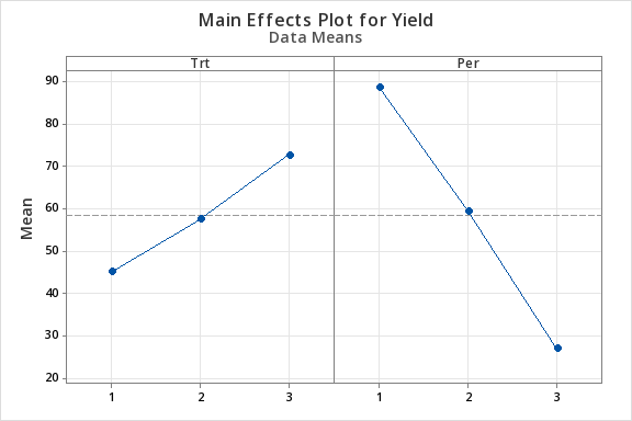{#fig-maineffectsyieldcow .mx-auto .d-block .lightbox fig-alt="Main effects plot for treatment and period." width="60%"}
::: minitab_output
### General Linear Model: Yield versus Per, Cow, Trt {.unnumbered .unlisted}
#### Factor Information
| Factor | Type | Levels | Values |
|:-------|:------|-------:|:-----------------|
| Per | Fixed | 3 | 1, 2, 3 |
| Cow | Fixed | 6 | 1, 2, 3, 4, 5, 6 |
| Trt | Fixed | 3 | 1, 2, 3 |
: {.w-auto .table-sm .row-header}
#### Analysis of Variance
| Source | DF | Seq SS | Contribution | Adj SS | Adj MS | F-Value | P-Value |
|:-------|----:|--------:|-------------:|--------:|-------:|--------:|--------:|
| Per | 2 | 11480.1 | 56.38% | 11480.1 | 5740.1 | 55.70 | 0.000 |
| Cow | 5 | 5781.1 | 28.39% | 5781.1 | 1156.2 | 11.22 | 0.002 |
| Trt | 2 | 2276.8 | 11.18% | 2276.8 | 1138.4 | 11.05 | 0.005 |
| Error | 8 | 824.4 | 4.05% | 824.4 | 103.1 | | |
| Total | 17 | 20362.4 | 100.00% | | | | |
: {.w-auto .table-sm .row-header}
#### Model Summary
| S | R-sq | R-sq(adj) | PRESS | R-sq(pred) | AICc | BIC |
|--------:|-------:|----------:|--------:|-----------:|-------:|-------:|
| 10.1516 | 95.95% | 91.40% | 4173.75 | 79.50% | 185.92 | 151.71 |
: {.w-auto .table-sm }
:::
So, let's go one step farther...
Is this an example of Case 2 or Case 3 of the multiple Latin Squares that we had looked at earlier?
This is a Case 2 where the column factor, the cows are nested within the square, but the row factor, period, is the same across squares.
Notice the sum of squares for cows is 5781.1. Let's change the model slightly using the general linear model in Minitab again. Follow along with the video.
The video demonstrations are based on Minitab v19.
```{=html}
<button class="btn btn-outline-success collapsed mb-3 ms-3" type="submit" data-bs-toggle="collapse" data-bs-target="#collapseExample3" aria-expanded="false" aria-controls="collapseExample3"> Step 2 Video Tutorial
</button>
```
::::: {#collapseExample3 .collapse}
:::: {.card .card-body}
::: {#vid-cowstep2 .w-75 .mx-auto}
{{< video https://youtu.be/omOFJi0YIk0 >}}
503 L4 Cow Step2
:::
::::
:::::
Now I want to move from Case 2 to Case 3. Is the period effect in the first square the same as the period effect in the second square? If it only means order and all the cows start lactating at the same time it might mean the same. But if some of the cows are done in the spring and others are done in the fall or summer, then the period effect has more meaning than simply the order. Although this represents order it may also involve other effects you need to be aware of this. A Case 3 approach involves estimating separate period effects within each square.
The video demonstrations are based on Minitab v19.
```{=html}
<button class="btn btn-outline-success collapsed mb-3 ms-3" type="submit" data-bs-toggle="collapse" data-bs-target="#collapseExample4" aria-expanded="false" aria-controls="collapseExample4"> Step 3 Video Tutorial
</button>
```
::::: {#collapseExample4 .collapse}
:::: {.card .card-body}
::: {#vid-cowstep3 .w-75 .mx-auto}
{{< video https://youtu.be/hLaMk0AwzGg >}}
503 L4 Cow Step3
:::
::::
:::::
My guess is that they all started the experiment at the same time - in this case, the first model would have been appropriate.
### How Do We Analyze Carryover Effect? {.unnumbered .unlisted}
OK, we are looking at the main treatment effects. With our first cow, during the first period, we give it a treatment or diet and we measure the yield. Obviously, you don't have any carryover effects here because it is the first period. However, what if the treatment they were first given was a really bad treatment? In fact in this experiment the diet A consisted of only roughage, so, the cow's health might in fact deteriorate as a result of this treatment. This could carry over into the next period. This carryover would hurt the second treatment if the washout period isn't long enough. The measurement at this point is a direct reflection of treatment B but may also have some influence from the previous treatment, treatment A.
If you look at how we have coded data here, we have another column called residual treatment. For the first six observations, we have just assigned this a value of 0 because there is no residual treatment. But for the first observation in the second row, we have labeled this with a value of one indicating that this was the treatment prior to the current treatment (treatment A). In this way the data is coded such that this column indicates the treatment given in the prior period for that cow.
Now we have another factor that we can put in our model. Let's take a look at how this looks in Minitab:
The video demonstrations are based on Minitab v19.
```{=html}
<button class="btn btn-outline-success collapsed mb-3 ms-3" type="submit" data-bs-toggle="collapse" data-bs-target="#collapseExample5" aria-expanded="false" aria-controls="collapseExample5"> Step 4 Video Tutorial
</button>
```
::::: {#collapseExample5 .collapse}
:::: {.card .card-body}
::: {#vid-cowstep4 .w-75 .mx-auto}
{{< video https://youtu.be/oz92SeQHWRA >}}
503 L4 Cow Step4
:::
::::
:::::
We have learned everything we need to learn. We have the appropriate analysis of variance here. By fitting in order, when residual treatment (i.e., ResTrt) was fit last we get:
::: ms-3
SS(treatment \| period, cow) = 2276.8\
SS(ResTrt \| period, cow, treatment) = 616.2
:::
When we flip the order of our treatment and residual treatment, we get the sums of squares due to fitting residual treatment after adjusting for period and cow:
::: ms-3
SS(ResTrt \| period, cow) = 38.4\
SS(treatment \| period, cow, ResTrt) = 2854.6
:::
Which of these are we interested in? If we wanted to test for residual treatment effects how would we do that? What would we use to test for treatment effects if we wanted to remove any carryover effects?
## Incomplete Block Designs
In using incomplete block designs we will use the notation *t* = \# of treatments. We define the block size as *k*. And, as you will see, in incomplete block designs *k* will be less than *t*. You cannot assign all of the treatments in each block. In short,
::: ms-3
*t* = \# of treatments,\
*k* = block size,\
*b* = \# of blocks,\
$r_i$ = \# of replicates for treatment i, in the entire design.
:::
Remember that an equal number of replications is the best way to be sure that you have minimum variance if you're looking at all possible pairwise comparisons. If $r_i = r$ for all treatments, the total number of observations in the experiment is *N* where:
$$N = t(r) = b(k)$$
The incidence matrix which defines the design of the experiment, gives the number of observations say $n_{ij}$ for the $i^{th}$ treatment in the $j^{th}$ block. This is what it might look like here:
::: {#fig-incompletesquare .bg-white .w-50 .mx-auto .d-block .mb-3}
```{=html}
<svg data-name="Layer 2" viewbox="0 0 238.62 219.16" xmlns="http://www.w3.org/2000/svg" id="svg2" role="img" aria-labelledby="title" > <title>A blank grid labeled to represent a general experimental design framework. Rows correspond to treatments numbered 1 to t, and columns correspond to blocks numbered 1 to b. Each cell is labeled with 𝑛_{ij}, representing the number of observations or measurements for the combination of treatment i and block j. Dots indicate the continuation of rows and columns. </title><path d="M48.12 45.32h190v173h-190z" fill="none" stroke="#000" stroke-miterlimit="10"></path><text font-size="18" transform="translate(58.88 37.07)">1</text><text font-size="18" transform="translate(95.88 37.07)">2</text><text font-size="18" transform="translate(157.84 37.07)">...</text><text font-size="18" transform="translate(218.51 37.07)">b</text><text font-size="18" transform="translate(26.88 69.07)">1</text><text font-size="18" transform="translate(26.88 110.07)">2</text><text font-size="18" transform="translate(28.85 212.07)">t</text><text font-size="18" transform="translate(29.63 133.07)">.</text><text font-size="18" transform="translate(29.63 154.07)">.</text><text font-size="18" transform="translate(29.63 175.07)">.</text><text font-size="13" transform="translate(123.2 11.14)">blocks</text><text font-size="12" transform="rotate(-90 86.37 76.09)">treatments</text><text font-size="15" transform="translate(16.52 25.8)">n</text><text font-size="15" transform="matrix(.58 0 0 .58 25.73 30.8)">ij</text></svg>
```
:::
Here we have treatments 1, 2, up to *t* and the blocks 1, 2, up to *b*. For a complete block design, we would have each treatment occurring one time within each block, so all entries in this matrix would be 1's. For an incomplete block design, the incidence matrix would be 0's and 1's simply indicating whether or not that treatment occurs in that block.
::::: {#exm-incidenceex1}
The example that we will look at is Table 4.22 (4.21 in 7th ed). Here is the incidence matrix for this example:
::: {#fig-incidencematrix1 .bg-white .w-25 .mx-auto .d-block .mb-3}
```{=html}
<svg viewbox="0 0 196.62 198.77" xmlns="http://www.w3.org/2000/svg" id="svg2" role="img" aria-labelledby="title" > <title> A 4x4 grid with rows and columns numbered 1 to 4. Each cell contains a binary value (0 or 1).</title><g data-name="Layer 2" fill="none" stroke="#000" stroke-miterlimit="10"><path d="M10.62 12.77h185v185h-185z" stroke-width="2"></path><path d="M57.62 12.77v185" stroke-width=".75"></path><path d="M103.62 12.77v185"></path><path d="M148.62 12.77v185M10.62 59.77h185" stroke-width=".75"></path><path d="M10.62 105.77h185"></path><path d="M10.62 150.77h185" stroke-width=".75"></path></g><g data-name="Layer 3"><text font-size="12" transform="translate(33.28 10.04)">1</text><text font-size="12" transform="translate(2.28 41.04)">1</text><text font-size="12" transform="translate(77.95 10.04)">2</text><text font-size="12" transform="translate(122.62 10.04)">3</text><text font-size="12" transform="translate(167.28 10.04)">4</text><text font-size="12" transform="translate(2.28 87.04)">2</text><text font-size="12" transform="translate(2.28 133.04)">3</text><text font-size="12" transform="translate(2.28 179.04)">4</text><text fill="#065094" font-size="18" transform="translate(28.48 43.43)">1</text><text fill="#065094" font-size="18" transform="translate(28.48 89.43)">0</text><text fill="#065094" font-size="18" transform="translate(28.48 134.43)">1</text><text fill="#065094" font-size="18" transform="translate(28.48 180.43)">1</text><text fill="#065094" font-size="18" transform="translate(73.82 43.43)">1</text><text fill="#065094" font-size="18" transform="translate(73.82 89.43)">1</text><text fill="#065094" font-size="18" transform="translate(73.82 134.43)">1</text><text fill="#065094" font-size="18" transform="translate(73.82 180.43)">0</text><text fill="#065094" font-size="18" transform="translate(119.15 43.43)">0</text><text fill="#065094" font-size="18" transform="translate(119.15 89.43)">1</text><text fill="#065094" font-size="18" transform="translate(119.15 134.43)">1</text><text fill="#065094" font-size="18" transform="translate(119.15 180.43)">1</text><text fill="#065094" font-size="18" transform="translate(164.48 43.43)">1</text><text fill="#065094" font-size="18" transform="translate(164.48 89.43)">1</text><text fill="#065094" font-size="18" transform="translate(164.48 134.43)">0</text><text fill="#065094" font-size="18" transform="translate(164.48 180.43)">1</text></g></svg>
```
:::
Here we have *t* = 4, *b* = 4, (four rows and four columns) and *k* = 3 ( so at each block we can only put three of the four treatments leaving one treatment out of each block). So, in this case, the row sums ($r_i$) and the columns sums, *k*, are all equal to 3.
::: {#fig-incidencematrix2 .bg-white .w-25 .mx-auto .d-block .mb-3}
```{=html}
<svg viewbox="0 0 215.35 219.31" xmlns="http://www.w3.org/2000/svg" id="svg2" role="img" aria-labelledby="title" >Matrix layout representing a 4x4 grid with numerical entries (1s and 0s) in each cell. The grid has labeled rows (1-4) on the left and labeled columns (1-4) on the top. Row and column sums are displayed as 3s along the right side and bottom of the grid. <title> </title><g data-name="Layer 2" fill="none" stroke="#000" stroke-miterlimit="10"><path d="M10.62 12.77h185v185h-185z" stroke-width="2"></path><path d="M57.62 12.77v185" stroke-width=".75"></path><path d="M103.62 12.77v185"></path><path d="M148.62 12.77v185M10.62 59.77h185" stroke-width=".75"></path><path d="M10.62 105.77h185"></path><path d="M10.62 150.77h185" stroke-width=".75"></path></g><g data-name="Layer 3"><text font-size="12" transform="translate(33.28 10.04)">1</text><text font-size="12" transform="translate(2.28 41.04)">1</text><text font-size="12" transform="translate(77.95 10.04)">2</text><text font-size="12" transform="translate(122.62 10.04)">3</text><text font-size="12" transform="translate(167.28 10.04)">4</text><text font-size="12" transform="translate(2.28 87.04)">2</text><text font-size="12" transform="translate(2.28 133.04)">3</text><text font-size="12" transform="translate(2.28 179.04)">4</text><text fill="#065094" font-size="18" transform="translate(28.48 43.43)">1</text><text fill="#065094" font-size="18" transform="translate(28.48 89.26)">0</text><text fill="#065094" font-size="18" transform="translate(28.48 134.5)">1</text><text fill="#065094" font-size="18" transform="translate(28.48 180.43)">1</text><text fill="#065094" font-size="18" transform="translate(73.82 43.43)">1</text><text fill="#065094" font-size="18" transform="translate(73.82 89.26)">1</text><text fill="#065094" font-size="18" transform="translate(73.82 134.5)">1</text><text fill="#065094" font-size="18" transform="translate(73.82 180.43)">0</text><text fill="#065094" font-size="18" transform="translate(119.15 43.43)">0</text><text fill="#065094" font-size="18" transform="translate(119.15 89.26)">1</text><text fill="#065094" font-size="18" transform="translate(119.15 134.5)">1</text><text fill="#065094" font-size="18" transform="translate(119.15 180.43)">1</text><text fill="#065094" font-size="18" transform="translate(164.48 43.43)">1</text><text fill="#065094" font-size="18" transform="translate(164.48 89.26)">1</text><text fill="#065094" font-size="18" transform="translate(164.48 134.5)">0</text><text fill="#065094" font-size="18" transform="translate(164.48 180.43)">1</text><text fill="#065094" font-size="18" transform="translate(199.48 43.43)">3</text><text fill="#065094" font-size="18" transform="translate(199.48 89.26)">3</text><text fill="#065094" font-size="18" transform="translate(199.48 134.5)">3</text><text fill="#065094" font-size="18" transform="translate(199.48 180.43)">3</text><text fill="#065094" font-size="18" transform="translate(28.48 214.43)">3</text><text fill="#065094" font-size="18" transform="translate(73.82 214.43)">3</text><text fill="#065094" font-size="18" transform="translate(119.15 214.43)">3</text><text fill="#065094" font-size="18" transform="translate(164.48 214.43)">3</text></g></svg>
```
:::
In general, we are faced with a situation where the number of treatments is specified, and the block size, or number of experimental units per block (*k*) is given. This is usually a constraint given from the experimental situation. And then, the researcher must decide how many blocks are needed to run and how many replicates that provides in order to achieve the precision or the power that you want for the test.
:::::
:::: {#exm-incidenceex2}
Here is another example of an incidence matrix for allocating treatments and replicates in an incomplete block design. Let's take an example where *k* = 2, still *t* = 4, and *b* = 4. That gives us a case *r* = 2. In This case we could design our incidence matrix so that it might look like this:
::: {#fig-incidencematrix3 .bg-white .w-25 .mx-auto .d-block .mb-3}
```{=html}
<svg viewbox="0 0 215.35 219.31" xmlns="http://www.w3.org/2000/svg" id="svg2" role="img" aria-labelledby="title" >Matrix layout showing a 4x4 grid with entries of 1s and 0s in the cells. Rows (1-4) are labeled on the left, and columns (1-4) are labeled at the top. Sums of each row and column are displayed as 2s, shown to the right of the rows and below the columns. <title> </title><g data-name="Layer 2" fill="none" stroke="#000" stroke-miterlimit="10"><path d="M10.62 12.77h185v185h-185z" stroke-width="2"></path><path d="M57.62 12.77v185" stroke-width=".75"></path><path d="M103.62 12.77v185"></path><path d="M148.62 12.77v185M10.62 59.77h185" stroke-width=".75"></path><path d="M10.62 105.77h185"></path><path d="M10.62 150.77h185" stroke-width=".75"></path></g><g data-name="Layer 3"><text font-size="12" transform="translate(33.28 10.04)">1</text><text font-size="12" transform="translate(2.28 41.04)">1</text><text font-size="12" transform="translate(77.95 10.04)">2</text><text font-size="12" transform="translate(122.62 10.04)">3</text><text font-size="12" transform="translate(167.28 10.04)">4</text><text font-size="12" transform="translate(2.28 87.04)">2</text><text font-size="12" transform="translate(2.28 133.04)">3</text><text font-size="12" transform="translate(2.28 179.04)">4</text><text fill="#065094" font-size="18" transform="translate(28.48 43.43)">1</text><text fill="#065094" font-size="18" transform="translate(28.48 89.26)">0</text><text fill="#065094" font-size="18" transform="translate(28.48 134.5)">1</text><text fill="#065094" font-size="18" transform="translate(28.48 180.43)">0</text><text fill="#065094" font-size="18" transform="translate(73.82 43.43)">0</text><text fill="#065094" font-size="18" transform="translate(73.82 89.26)">1</text><text fill="#065094" font-size="18" transform="translate(73.82 134.5)">0</text><text fill="#065094" font-size="18" transform="translate(73.82 180.43)">1</text><text fill="#065094" font-size="18" transform="translate(119.15 43.43)">1</text><text fill="#065094" font-size="18" transform="translate(119.15 89.26)">0</text><text fill="#065094" font-size="18" transform="translate(119.15 134.5)">1</text><text fill="#065094" font-size="18" transform="translate(119.15 180.43)">0</text><text fill="#065094" font-size="18" transform="translate(164.48 43.43)">0</text><text fill="#065094" font-size="18" transform="translate(164.48 89.26)">1</text><text fill="#065094" font-size="18" transform="translate(164.48 134.5)">0</text><text fill="#065094" font-size="18" transform="translate(164.48 180.43)">1</text><text fill="#065094" font-size="18" transform="translate(199.48 43.43)">2</text><text fill="#065094" font-size="18" transform="translate(199.48 89.26)">2</text><text fill="#065094" font-size="18" transform="translate(199.48 134.5)">2</text><text fill="#065094" font-size="18" transform="translate(199.48 180.43)">2</text><text fill="#065094" font-size="18" transform="translate(28.48 214.43)">2</text><text fill="#065094" font-size="18" transform="translate(73.82 214.43)">2</text><text fill="#065094" font-size="18" transform="translate(119.15 214.43)">2</text><text fill="#065094" font-size="18" transform="translate(164.48 214.43)">2</text></g></svg>
```
:::
This example has two observations per block so *k* = 2 in each case and for all treatments *r* = 2.
::::
### Balanced Incomplete Block Design (BIBD) {.unnumbered .unlisted}
A BIBD is an incomplete block design where all pairs of treatments occur together within a block an equal number of times ( \$\lambda) ). In general, we will specify $\lambda_{ii^\prime}$ as the number of times treatment $i$ occurs with $i^\prime$, in a block.
Let's look at previous cases. How many times does treatment one and two occur together in this first example design?
::: {#fig-balancedblock .bg-white .w-25 .mx-auto .d-block .mb-3}
```{=html}
<svg viewbox="0 0 233.87 236.18" xmlns="http://www.w3.org/2000/svg" id="svg2" role="img" aria-labelledby="title" >4x4 matrix illustrating treatments and blocks in a balanced experimental design. The rows represent treatments, and the columns represent blocks. Each cell contains either a 1 or 0, denoting treatment assignments. Rows and columns are labeled, with their respective totals (3s) displayed along the margins. Highlighted cells in light blue represent specific assignments within blocks 2 and 4. <title> </title><g data-name="Layer 5" fill="#aadcdf"><path d="M76.14 29.06h46v93h-46zM167.14 29.06h46v93h-46z"></path></g><g data-name="Layer 2" fill="none" stroke="#000" stroke-miterlimit="10"><path d="M29.14 29.25h185v185h-185z" stroke-width="2"></path><path d="M76.14 29.25v185" stroke-width=".75"></path><path d="M122.14 29.25v185"></path><path d="M167.14 29.25v185M29.14 76.25h185" stroke-width=".75"></path><path d="M29.14 122.25h185"></path><path d="M29.14 167.25h185" stroke-width=".75"></path></g><g data-name="Layer 3" font-family="OpenSans-Bold, Open Sans" font-weight="700"><text font-size="14" transform="translate(50.89 26.64)">1</text><text font-size="14" transform="translate(17.89 59.64)">1</text><text font-size="14" transform="translate(95.55 26.64)">2</text><text font-size="14" transform="translate(140.22 26.64)">3</text><text font-size="14" transform="translate(184.89 26.64)">4</text><text font-size="14" transform="translate(17.89 105.64)">2</text><text font-size="14" transform="translate(17.89 151.64)">3</text><text font-size="14" transform="translate(17.89 197.64)">4</text><text fill="#172741" font-size="18" transform="translate(47.01 59.91)">1</text><text fill="#172741" font-size="18" transform="translate(47.01 105.74)">0</text><text fill="#172741" font-size="18" transform="translate(47.01 150.97)">1</text><text fill="#172741" font-size="18" transform="translate(47.01 196.91)">1</text><text fill="#172741" font-size="18" transform="translate(92.35 59.91)">1</text><text fill="#172741" font-size="18" transform="translate(92.35 105.74)">1</text><text fill="#172741" font-size="18" transform="translate(92.35 150.97)">1</text><text fill="#172741" font-size="18" transform="translate(92.35 196.91)">0</text><text fill="#172741" font-size="18" transform="translate(137.68 59.91)">0</text><text fill="#172741" font-size="18" transform="translate(137.68 105.74)">1</text><text fill="#172741" font-size="18" transform="translate(137.68 150.97)">1</text><text fill="#172741" font-size="18" transform="translate(137.68 196.91)">1</text><text fill="#172741" font-size="18" transform="translate(183.01 59.91)">1</text><text fill="#172741" font-size="18" transform="translate(183.01 105.74)">1</text><text fill="#172741" font-size="18" transform="translate(183.01 150.97)">0</text><text fill="#172741" font-size="18" transform="translate(183.01 196.91)">1</text><text fill="#172741" font-size="18" transform="translate(218.01 59.91)">3</text><text fill="#172741" font-size="18" transform="translate(218.01 105.74)">3</text><text fill="#172741" font-size="18" transform="translate(218.01 150.97)">3</text><text fill="#172741" font-size="18" transform="translate(218.01 196.91)">3</text><text fill="#172741" font-size="18" transform="translate(47.01 230.91)">3</text><text fill="#172741" font-size="18" transform="translate(92.35 230.91)">3</text><text fill="#172741" font-size="18" transform="translate(137.68 230.91)">3</text><text fill="#172741" font-size="18" transform="translate(183.01 230.91)">3</text></g><g data-name="Layer 4" font-family="OpenSans-Bold, Open Sans" font-size="12" font-weight="700"><text transform="translate(97.27 10.28)">blocks</text><text transform="rotate(-90 83.67 73.39)">treatments</text></g></svg>
```
:::
It occurs together in block 2 and then again in block 4 (highlighted in light blue). So, $\lambda_{12} = 2$. If we look at treatment one and three, this occurs together in block one and in block two therefore $\lambda_{13} = 2$. In this design, you can look at all possible pairs. Let's look at 1 and 4 - they occur together twice, 2 and 3 occur together twice, 2 and 4 twice, and 3 and 4 occur together twice. For this design $\lambda_{ii^\prime} = 2$ for all $ii^\prime$ treatment pairs defining the concept of balance in this incomplete block design.
If the number of times treatments occur together within a block is equal across the design for all pairs of treatments then we call this a balanced incomplete block design (BIBD).
Now look at the incidence matrix for the second example.
::: {#fig-bibd .bg-white .w-25 .mx-auto .d-block .mb-3}
```{=html}
<svg viewbox="0 0 215.35 219.31" xmlns="http://www.w3.org/2000/svg" id="svg2" role="img" aria-labelledby="title" >Matrix layout showing a 4x4 grid with entries of 1s and 0s in the cells. Rows (1-4) are labeled on the left, and columns (1-4) are labeled at the top. Sums of each row and column are displayed as 2s, shown to the right of the rows and below the columns. <title> </title><g data-name="Layer 2" fill="none" stroke="#000" stroke-miterlimit="10"><path d="M10.62 12.77h185v185h-185z" stroke-width="2"></path><path d="M57.62 12.77v185" stroke-width=".75"></path><path d="M103.62 12.77v185"></path><path d="M148.62 12.77v185M10.62 59.77h185" stroke-width=".75"></path><path d="M10.62 105.77h185"></path><path d="M10.62 150.77h185" stroke-width=".75"></path></g><g data-name="Layer 3"><text font-size="12" transform="translate(33.28 10.04)">1</text><text font-size="12" transform="translate(2.28 41.04)">1</text><text font-size="12" transform="translate(77.95 10.04)">2</text><text font-size="12" transform="translate(122.62 10.04)">3</text><text font-size="12" transform="translate(167.28 10.04)">4</text><text font-size="12" transform="translate(2.28 87.04)">2</text><text font-size="12" transform="translate(2.28 133.04)">3</text><text font-size="12" transform="translate(2.28 179.04)">4</text><text fill="#065094" font-size="18" transform="translate(28.48 43.43)">1</text><text fill="#065094" font-size="18" transform="translate(28.48 89.26)">0</text><text fill="#065094" font-size="18" transform="translate(28.48 134.5)">1</text><text fill="#065094" font-size="18" transform="translate(28.48 180.43)">0</text><text fill="#065094" font-size="18" transform="translate(73.82 43.43)">0</text><text fill="#065094" font-size="18" transform="translate(73.82 89.26)">1</text><text fill="#065094" font-size="18" transform="translate(73.82 134.5)">0</text><text fill="#065094" font-size="18" transform="translate(73.82 180.43)">1</text><text fill="#065094" font-size="18" transform="translate(119.15 43.43)">1</text><text fill="#065094" font-size="18" transform="translate(119.15 89.26)">0</text><text fill="#065094" font-size="18" transform="translate(119.15 134.5)">1</text><text fill="#065094" font-size="18" transform="translate(119.15 180.43)">0</text><text fill="#065094" font-size="18" transform="translate(164.48 43.43)">0</text><text fill="#065094" font-size="18" transform="translate(164.48 89.26)">1</text><text fill="#065094" font-size="18" transform="translate(164.48 134.5)">0</text><text fill="#065094" font-size="18" transform="translate(164.48 180.43)">1</text><text fill="#065094" font-size="18" transform="translate(199.48 43.43)">2</text><text fill="#065094" font-size="18" transform="translate(199.48 89.26)">2</text><text fill="#065094" font-size="18" transform="translate(199.48 134.5)">2</text><text fill="#065094" font-size="18" transform="translate(199.48 180.43)">2</text><text fill="#065094" font-size="18" transform="translate(28.48 214.43)">2</text><text fill="#065094" font-size="18" transform="translate(73.82 214.43)">2</text><text fill="#065094" font-size="18" transform="translate(119.15 214.43)">2</text><text fill="#065094" font-size="18" transform="translate(164.48 214.43)">2</text></g></svg>
```
:::
We can see that:
| $\lambda_{12}$ occurs together 0 times.
| $\lambda_{13}$ occurs together 2 times.
| $\lambda_{14}$ occurs together 0 times.
| $\lambda_{23}$ occurs together 0 times.
| $\lambda_{24}$ occurs together 2 times.
| $\lambda_{34}$ occurs together to 0 times.
Here we have two pairs occurring together 2 times and the other four pairs occurring together 0 times. Therefore, this is not a balanced incomplete block design (BIBD).
### What else is there about BIBD? {.unnumbered .unlisted}
We can define $\lambda$ in terms of our design parameters when we have equal block size k, and equal replication $r_i = r$. For a given set of t, k, and r we define $\lambda$ as:
| $\lambda = r(k-1) / t-1$
\
So, for the first example that we looked at earlier - let's plug in the values and calculate $\lambda:$
| $\lambda = 3 (3 - 1) / (4 -1) = 2$
\
Here is the key: when $\lambda$ is equal to an integer number it tells us that a balanced incomplete block design exists. Let's look at the second example and use the formula and plug in the values for this second example. So, for $t = 4,$ $k = 2,$ $r = 2,$ and $b = 4,$ we have:
| $\lambda = 2 (2 - 1) / (4 - 1) = 0.666$
\
Since $\lambda$ is not an integer there does not exist a balanced incomplete block design for this experiment. We would either need more replicates or a larger block size. Seeing as how the block size in this case is fixed, we can achieve a balanced complete block design by adding more replicates so that $\lambda$ equals at least 1. It needs to be a whole number in order for the design to be balanced.
We will talk about partially balanced designs later. But in thinking about this case we note that a balanced design doesn't exist so what would be the best partially balanced design? That would be a question that you would ask if you could only afford four blocks and the block size is two. Given this situation, is the design in Example 2 the best design we can construct? The best partially balanced design is where $\lambda_{ii^\prime}$ should be the nearest integers to the $\lambda$ that we calculated. In our case each $\lambda_{ii^\prime}$ should be either 0 or 1, the integers nearest 0.667. This example is not as close to balanced as it could be. In fact, it is not even a connected design where you can go from any treatment to any other treatment within a block. More about this later...
### How do you construct a BIBD? {.unnumbered .unlisted}
In some situations, it is easy to construct the best IBD, however, for other cases it can be quite difficult and we will look them up in a reference.
Let's say that we want six blocks, we still want 4 treatments and our block size is still 2. Calculate $\lambda = r(k - 1) / (t - 1) = 1$. We want to create all possible pairs of treatments because lambda is equal to one. We do this by looking at all possible combinations of four treatments taking two at a time. We could set up the incidence matrix for the design or we could represent it like this - entries in the table are treatment labels: {1, 2, 3, 4}.
::: {#fig-bibd2 .bg-white .w-50 .mx-auto .d-block .mb-3}
```{=html}
<svg viewbox="0 0 269.52 97.97" xmlns="http://www.w3.org/2000/svg" id="svg2" role="img" aria-labelledby="title" > <title>2x6 matrix illustrating treatment assignments across six blocks. Rows represent treatment groups, and columns represent blocks. Each cell contains a numeric value (1–4) indicating treatment assignments. </title><g data-name="Layer 2" fill="none" stroke="#000" stroke-miterlimit="10"><path d="M11.02 10.47h258v87h-258zM11.02 54.47h258M55.02 10.47v87M98.02 10.47v87M141.02 10.47v87M183.02 10.47v87M226.02 10.47v87"></path></g><g data-name="Layer 3" font-weight="700"><text fill="#065094" font-size="18" transform="translate(27.46 40.23)">1</text><text fill="#065094" font-size="18" transform="translate(69.73 40.23)">1</text><text fill="#065094" font-size="18" transform="translate(112.32 40.23)">1</text><text fill="#065094" font-size="18" transform="translate(155.59 40.23)">2</text><text fill="#065094" font-size="18" transform="translate(197.86 40.23)">2</text><text fill="#065094" font-size="18" transform="translate(241.46 40.23)">3</text><text fill="#065094" font-size="18" transform="translate(27.46 83.23)">2</text><text fill="#065094" font-size="18" transform="translate(69.73 83.23)">3</text><text fill="#065094" font-size="18" transform="translate(112.33 83.23)">4</text><text fill="#065094" font-size="18" transform="translate(155.59 83.23)">3</text><text fill="#065094" font-size="18" transform="translate(197.86 83.23)">4</text><text fill="#065094" font-size="18" transform="translate(241.46 83.23)">4</text><text font-size="10" transform="translate(29.74 8.57)">1</text><text font-size="10" transform="translate(72.01 8.57)">2</text><text font-size="10" transform="translate(114.61 8.57)">3</text><text font-size="10" transform="translate(157.87 8.57)">4</text><text font-size="10" transform="translate(200.14 8.57)">5</text><text font-size="10" transform="translate(243.74 8.57)">6</text><text font-size="10" transform="translate(2.9 38.54)">1</text><text font-size="10" transform="translate(2.9 81.54)">2</text></g></svg>
```
:::
However, this method of constructing a BIBD using all possible combinations, does not always work as we now demonstrate. If the number of combinations is too large then you need to find a subset - - not always easy to do. However, sometimes you can use Latin Squares to construct a BIBD. As an example, let's take any 3 columns from a 4 × 4 Latin Square design. This subset of columns from the whole Latin Square creates a BIBD. However, not every subset of a Latin Square is a BIBD.
Let's look at an example. In this example we have $t = 7,$ $b = 7,$ and $k = 3.$ This means that $r = 3 = (bk) / t.$ Here is the 7 × 7 Latin square:
::: {#fig-latinsqu7x7 .bg-white .w-25 .mx-auto .d-block .mb-3}
```{=html}
<svg viewbox="0 0 223 223" xmlns="http://www.w3.org/2000/svg" id="svg2" role="img" aria-labelledby="title" > <title> a 7x7 Latin square, a statistical design tool where each treatment (A through G) appears exactly once in each row and column. The parameters are t=7,b=7, k=3, leading to r=3 repetitions per treatment.</title><g data-name="Layer 2" fill="none" stroke="#000" stroke-miterlimit="10"><path d="M1 128h221M1 159h221M1 191h221"></path><path d="M1 1h221v221H1z" stroke-width="2"></path><path d="M1 34h221M1 65h221M1 96h221M34 1v221M65 0v221M96 0v221M127 0v221M159 1v221M190 1v221"></path></g><g data-name="Layer 3" fill="#065094" font-size="18" font-weight="700"><text transform="translate(12.22 25.42)">A</text><text transform="translate(42.07 25.42)">B</text><text transform="translate(73.69 25.42)">C</text><text transform="translate(104.74 25.42)">D</text><text transform="translate(137.15 25.42)">E</text><text transform="translate(168.56 25.42)">F</text><text transform="translate(198.29 25.42)">G</text><text transform="translate(12.38 56.51)">B</text><text transform="translate(42.38 56.51)">C</text><text transform="translate(72.77 56.51)">D</text><text transform="translate(106.36 56.51)">E</text><text transform="translate(137.25 56.51)">F</text><text transform="translate(166.98 56.51)">G</text><text transform="translate(198.6 56.51)">A</text><text transform="translate(12.69 87.59)">C</text><text transform="translate(41.46 87.59)">D</text><text transform="translate(74.39 87.59)">E</text><text transform="translate(106.47 87.59)">F</text><text transform="translate(135.67 87.59)">G</text><text transform="translate(167.29 87.59)">A</text><text transform="translate(198.76 87.59)">B</text><text transform="translate(11.77 118.67)">D</text><text transform="translate(43.08 118.67)">E</text><text transform="translate(74.49 118.67)">F</text><text transform="translate(104.89 118.67)">G</text><text transform="translate(135.98 118.67)">A</text><text transform="translate(167.45 118.67)">B</text><text transform="translate(199.07 118.67)">C</text><text transform="translate(13.39 149.76)">E</text><text transform="translate(43.18 149.76)">F</text><text transform="translate(72.91 149.76)">G</text><text transform="translate(105.2 149.76)">A</text><text transform="translate(136.14 149.76)">B</text><text transform="translate(167.76 149.76)">C</text><text transform="translate(198.15 149.76)">D</text><text transform="translate(13.49 180.84)">F</text><text transform="translate(41.6 180.84)">G</text><text transform="translate(73.22 180.84)">A</text><text transform="translate(105.36 180.84)">B</text><text transform="translate(136.46 180.84)">C</text><text transform="translate(166.84 180.84)">D</text><text transform="translate(199.77 180.84)">E</text><text transform="translate(11.91 211.92)">G</text><text transform="translate(41.91 211.92)">A</text><text transform="translate(73.38 211.92)">B</text><text transform="translate(105.67 211.92)">C</text><text transform="translate(135.53 211.92)">D</text><text transform="translate(168.46 211.92)">E</text><text transform="translate(199.87 211.92)">F</text></g></svg>
```
:::
We want to select ($k = 3$) three columns out of this design where each treatment occurs once with every other treatment because $\lambda = 3(3 - 1) / (7 - 1) = 1$.
We could select the first three columns - let's see if this will work. Click the animation below to see whether using the first three columns would give us combinations of treatments where treatment pairs are not repeated.
```{=html}
<p><iframe allowfullscreen="allowfullscreen" frameborder="0" height="auto" src="https://h5p.org/h5p/embed/549117" width="100%"></iframe><script src="https://h5p.org/sites/all/modules/h5p/library/js/h5p-resizer.js" charset="UTF-8"></script></p>
```
Since the first three columns contain some pairs more than once, let's try columns 1, 2, and now we need a third...how about the fourth column. If you look at all possible combinations in each row, each treatment pair occurs only one time.
What if we could afford a block size of 4 instead of 3? Here *t* = 7, *b* = 7, *k* = 4, then *r* = 4. We calculate $\lambda = r(k - 1) / (t - 1) = 2$ so a BIBD does exist. For this design with a block size of 4 we can select 4 columns (or rows) from a Latin square. Let's look at columns again... can you select the correct 4?
Now consider the case with 8 treatments. The number of possible combinations of 8 treatments taking 4 at a time is 70. Thus with 70 sets of 4 from which you have to choose 14 blocks - - wow, this is a big job! At this point, we should simply look at an appropriate reference. Here is a handout - [a catalog that will help you with this selection process](/onlinecourses/sites/stat503/files/lesson04/Cochran_Cox.pdf) - taken from Cochran & Cox, *Experimental Design*, p. 469-482.
### Analysis of BIBD's {.unnumbered .unlisted}
When we have missing data, it affects the average of the remaining treatments in a row, i.e., when complete data does not exist for each row - this affects the means. When we have complete data the block effect and the column effects both drop out of the analysis since they are orthogonal. With missing data or IBDs that are not orthogonal, even BIBD where orthogonality does not exist, the analysis requires us to use GLM which codes the data like we did previously. The GLM fits first the block and then the treatment.
The sequential sums of squares (Seq SS) for block is not the same as the Adj SS.
We have the following:
::::: grid
::: {.g-col-lg-6 .g-col-md-6 .g-col-sm-12}
**Seq SS**\
$SS(\beta | \mu) 55.0$
$SS(\tau | \mu, \beta) = 22.50$
:::
::: {.g-col-lg-6 .g-col-md-6 .g-col-sm-12}
**Adj SS**\
$SS(\beta | \mu, \tau) = 66.08$
$SS(\tau | \mu, \beta) = 22.75$
:::
:::::
Switch them around...now first fit treatments and then the blocks.
::::: grid
::: {.g-col-lg-6 .g-col-md-6 .g-col-sm-12}
**Seq SS**\
$SS(\tau | \mu) = 11.67$
$SS(\beta | \mu, \tau) = 66.08$
:::
::: {.g-col-lg-6 .g-col-md-6 .g-col-sm-12}
**Adj SS**\
$SS(\tau | \mu, \beta) = 22.75$
$SS(\beta | \mu, \tau_i) = 66.08$
:::
:::::
The 'least squares means' come from the fitted model. Regardless of the pattern of missing data or the design we can conceptually think of our design represented by the model:
$$Y_{ij}= \mu + +\beta _{i}+\tau _{j}+e_{ij}$$
$i = 1, \dots , b, j= 1, \dots , t$
You can obtain the 'least squares means' from the estimated parameters from the least squares fit of the model.
## Optional Section {.unnumbered}
### SAS Code {.unnumbered}
{.d-block .float-end fig-alt="SAS logo" width="10%" .ps-3}
See the discussion in the text for Recovery of Interblock Information, p. 154. This refers to a procedure which allows us to extract additional information from a BIBD when the blocks are a random effect. Optionally you can read this section. We illustrate the analysis by the use of the software, `PROC` Mixed in SAS.
```SAS
data; input blk trt Y; cards;
1 1 73
1 3 73
1 4 75
2 1 74
2 2 75
2 3 75
3 2 67
3 3 68
3 4 72
4 1 71
4 2 72
4 4 75
;;;;
/*This data is from Example 4-5 in Montgomery, Design and Analysis of experiments, 6th edition, */
/* Wiley, 2005, pages 147-154.  This demonstrates the recovery of interblock information when   */
/* the blocks are considered random.  */
proc glm; class trt blk;
model Y = blk trt;
lsmeans trt/ e stderr pdiff;

proc mixed; class trt blk;
model Y = trt;
random blk;
lsmeans trt/ e pdiff;
/* The next 4 estimate statements calculate the treatment effects from the solution*/
estimate "trt effect 1" trt +.75 -.25 -.25 -.25/e;
estimate "trt effect 2" trt -.25 +.75 -.25 -.25/e;
estimate "trt effect 3" trt -.25 -.25 +.75 -.25/e;
estimate "trt effect 4" trt -.25 -.25 -.25 +.75/e;
/* The next 3 contrast statements show one set of orthogonal contrasts*/
contrast "trt1 vs trt2-4" trt 3 -1 -1 -1;
contrast "trt2 vs trt3-4" trt 0 2 -1 -1 ;
contrast "trt3 vs trt4" trt 0 0 1 -1 ;
run;
```
Note that the least squares means for treatments when using `PROC` Mixed, correspond to the combined intra- and inter-block estimates of the treatment effects.
#### Inspect the Code
Here the `PROC MIXED` procedure, includes a random block effect to provide recovery of interblock information.
Using the formula $\mu_i=\mu+\tau_i$, thus $\tau_i=\mu_i-\mu$ and $\mu=\frac{1}{4}(\mu_1+\mu_2+\mu_3+\mu_4)$
::: {.ms-2 .border-start .p-3 .border-primary}
```SAS
/* The next 4 estimate statements calculate the treatment effects from the solution*/
estimate "trt effect 1" trt +.75 -.25 -.25 -.25/e;
estimate "trt effect 2" trt -.25 +.75 -.25 -.25/e;
estimate "trt effect 3" trt -.25 -.25 +.75 -.25/e;
estimate "trt effect 4" trt -.25 -.25 -.25 +.75/e;
```
:::
When we run this program we get the following results...
quarto-executable-code-5450563D
```r
#| echo: false
sas_output <- sas_run_string("data; input blk trt Y; cards;
1 1 73
1 3 73
1 4 75
2 1 74
2 2 75
2 3 75
3 2 67
3 3 68
3 4 72
4 1 71
4 2 72
4 4 75
;;;;
/*This data is from Example 4-5 in Montgomery, Design and Analysis of experiments, 6th edition, */
/* Wiley, 2005, pages 147-154. This demonstrates the recovery of interblock information when */
/* the blocks are considered random. */
proc glm; class trt blk;
model Y = blk trt;
lsmeans trt/ e stderr pdiff;
proc mixed; class trt blk;
model Y = trt;
random blk;
lsmeans trt/ e pdiff;
/* The next 4 estimate statements calculate the treatment effects from the solution*/
estimate 'trt effect 1' trt +.75 -.25 -.25 -.25/e;
estimate 'trt effect 2' trt -.25 +.75 -.25 -.25/e;
estimate 'trt effect 3' trt -.25 -.25 +.75 -.25/e;
estimate 'trt effect 4' trt -.25 -.25 -.25 +.75/e;
/* The next 3 contrast statements show one set of orthogonal contrasts*/
contrast 'trt1 vs trt2-4' trt 3 -1 -1 -1;
contrast 'trt2 vs trt3-4' trt 0 2 -1 -1 ;
contrast 'trt3 vs trt4' trt 0 0 1 -1 ;
run;
/* Adding comments to the output */
data _null_;
put Note: The above output shows the pairwise comparisons with p-values.;
run;")
```
```{=html}
<details><summary>See complete SAS output</summary>
```
quarto-executable-code-5450563D
```r
#| echo: false
sas_output
```
```{=html}
</details>
```
::::: grid
::: {.g-col-lg-6 .g-col-md-6 .g-col-sm-12 .align-self-center}
Here we see that the Type I Sum of Squares are Sequential SS's:
:::
::: {.g-col-lg-6 .g-col-md-6 .g-col-sm-12}
quarto-executable-code-5450563D
```r
#| echo: false
sas_run_string("data; input blk trt Y; cards;
1 1 73
1 3 73
1 4 75
2 1 74
2 2 75
2 3 75
3 2 67
3 3 68
3 4 72
4 1 71
4 2 72
4 4 75
;;;;
options nodate nonumber; /* Suppress date and page numbers */
title; /* Clears any custom titles */
ods noptitles; /* Suppress procedure titles */
ods select ModelANOVA; /* Restrict output to Model ANOVA table */
proc glm;
class trt blk;
model Y = blk trt / ss1; /* Request Type I SS */
run;")
```
:::
:::::
::::: grid
::: {.g-col-lg-6 .g-col-md-6 .g-col-sm-12 .align-self-center}
Type III SS's are adjusted SS's adjusted for all other factors in the model:
:::
::: {.g-col-lg-6 .g-col-md-6 .g-col-sm-12}
quarto-executable-code-5450563D
```r
#| echo: false
sas_run_string("
data; input blk trt Y; cards;
1 1 73
1 3 73
1 4 75
2 1 74
2 2 75
2 3 75
3 2 67
3 3 68
3 4 72
4 1 71
4 2 72
4 4 75
;;;;
options nodate nonumber; /* Suppress date and page numbers */
title; /* Clears any custom titles */
ods noptitles; /* Suppress procedure titles */
ods select ModelANOVA; /* Restrict output to Model ANOVA table */
proc glm;
class trt blk;
model Y = blk trt / ss3; /* Request Type I SS */
run;")
```
:::
:::::
::::: grid
::: {.g-col-lg-6 .g-col-md-6 .g-col-sm-12 .align-self-center}
The F-values for trt in both tables are the intrablock analysis.
The intrablock analysis - adjusted means can be found in the `Y LSMEAN` column in the following table.
:::
::: {.g-col-lg-6 .g-col-md-6 .g-col-sm-12}
quarto-executable-code-5450563D
```r
#| echo: false
sas_run_string("
data example;
input blk trt Y;
cards;
1 1 73
1 3 73
1 4 75
2 1 74
2 2 75
2 3 75
3 2 67
3 3 68
3 4 72
4 1 71
4 2 72
4 4 75
;;;;
options nodate nonumber; /* Suppress date and page numbers */
title; /* Clear custom titles */
ods noptitles; /* Suppress procedure titles */
ods select IntrablockANOVA LSMeans; /* Select Intrablock Analysis and LSMeans tables */
proc glm;
class trt blk;
model Y = blk trt / ss3; /* Explicitly request Type III SS */
lsmeans trt / e stderr pdiff; /* Calculate LSMeans for treatments */
run;")
```
:::
:::::
::::: grid
::: {.g-col-lg-6 .g-col-md-6 .g-col-sm-12 .align-self-center}
Here we see the p-values for the pairwise tests...
:::
::: {.g-col-lg-6 .g-col-md-6 .g-col-sm-12}
quarto-executable-code-5450563D
```r
#| echo: false
sas_run_string("
data;
input blk trt Y;
cards;
1 1 73
1 3 73
1 4 75
2 1 74
2 2 75
2 3 75
3 2 67
3 3 68
3 4 72
4 1 71
4 2 72
4 4 75
;;;;
/* GLM Procedure */
proc glm;
class trt blk;
model Y = blk trt;
lsmeans trt / pdiff=all adjust=tukey; /* Only show pairwise comparisons */
ods select Diff;
run;")
```
:::
:::::
::::: grid
::: {.g-col-lg-6 .g-col-md-6 .g-col-sm-12 .align-self-center}
This table shows the $\sigma_\hat{2b}$ and $\sigma_\hat{2}$.
:::
::: {.g-col-lg-6 .g-col-md-6 .g-col-sm-12}
quarto-executable-code-5450563D
```r
#| echo: false
sas_run_string("
data;
input blk trt Y;
cards;
1 1 73
1 3 73
1 4 75
2 1 74
2 2 75
2 3 75
3 2 67
3 3 68
3 4 72
4 1 71
4 2 72
4 4 75
;;;;
/* GLM Procedure */
proc mixed; class trt blk;
model Y = trt;
random blk;
lsmeans trt/ e pdiff;
ods select CovParms;
run;")
```
:::
:::::
::::: grid
::: {.g-col-lg-6 .g-col-md-6 .g-col-sm-12 .align-self-center}
Comined estimates of $\tau_i$
:::
::: {.g-col-lg-6 .g-col-md-6 .g-col-sm-12}
quarto-executable-code-5450563D
```r
#| echo: false
sas_run_string("
data;
input blk trt Y;
cards;
1 1 73
1 3 73
1 4 75
2 1 74
2 2 75
2 3 75
3 2 67
3 3 68
3 4 72
4 1 71
4 2 72
4 4 75
;;;;
/* GLM Procedure */
proc mixed; class trt blk;
model Y = trt;
random blk;
lsmeans trt/ e pdiff;
estimate 'trt effect 1' trt +.75 -.25 -.25 -.25/e;
estimate 'trt effect 2' trt -.25 +.75 -.25 -.25/e;
estimate 'trt effect 3' trt -.25 -.25 +.75 -.25/e;
estimate 'trt effect 4' trt -.25 -.25 -.25 +.75/e;
ods select Estimates;
run;")
```
:::
:::::
::::: grid
::: {.g-col-lg-6 .g-col-md-6 .g-col-sm-12 .align-self-center}
Combined intra- and interblock estimates of the means...
:::
::: {.g-col-lg-6 .g-col-md-6 .g-col-sm-12}
quarto-executable-code-5450563D
```r
#| echo: false
sas_run_string("
data;
input blk trt Y;
cards;
1 1 73
1 3 73
1 4 75
2 1 74
2 2 75
2 3 75
3 2 67
3 3 68
3 4 72
4 1 71
4 2 72
4 4 75
;;;;
/* GLM Procedure */
proc mixed; class trt blk;
model Y = trt;
random blk;
lsmeans trt/ e pdiff;
estimate 'trt effect 1' trt +.75 -.25 -.25 -.25/e;
estimate 'trt effect 2' trt -.25 +.75 -.25 -.25/e;
estimate 'trt effect 3' trt -.25 -.25 +.75 -.25/e;
estimate 'trt effect 4' trt -.25 -.25 -.25 +.75/e;
ods select LSmeans;
run;")
```
:::
:::::
### Random Effect Factor {.unnumbered}
So far we have discussed experimental designs with fixed factors, that is, the levels of the factors are fixed and constrained to some specific values. However, this is often not the case. In some cases, the levels of the factors are selected at random from a larger population. In this case, the inference made on the significance of the factor can be extended to the whole population but the factor effects are treated as contributions to variance.
Minitab’s General Linear Command handles random factors appropriately as long as you are careful to select which factors are fixed and which are random.


